Load the Data

Load and plot the Australian CPI data.

loadData_JAustraliany = DataTable.PAU; T = length(y); figure plot(y) h1 = gca; h1.XLim = [0,T]; h1.XTick = 1:10:T; h1.XTickLabel = datestr(dates(1:10:T),17); title('Log Quarterly Australian CPI')

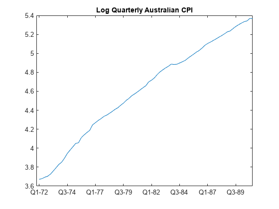
The series is nonstationary, with a clear upward trend.

Plot the Sample ACF and PACF

Plot the sample autocorrelation function (ACF) and partial autocorrelation function (PACF) for the CPI series.

figure subplot(2,1,1) autocorr(y) subplot(2,1,2) parcorr(y)

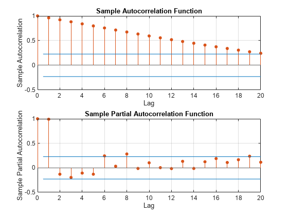
英蒂ACF显著,线性衰减的样本cates a nonstationary process.

Difference the Data

Take a first difference of the data, and plot the differenced series.

dY = diff(y); figure plot(dY) h2 = gca; h2.XLim = [0,T]; h2.XTick = 1:10:T; h2.XTickLabel = datestr(dates(2:10:T),17); title('Differenced Log Quarterly Australian CPI')

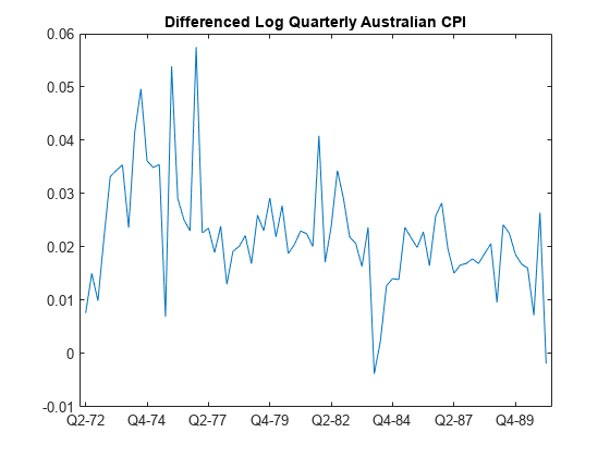
Differencing removes the linear trend. The differenced series appears more stationary.

Plot the Sample ACF and PACF of the Differenced Series

Plot the sample ACF and PACF of the differenced series to look for behavior more consistent with a stationary process.

figure subplot(2,1,1) autocorr(dY) subplot(2,1,2) parcorr(dY)

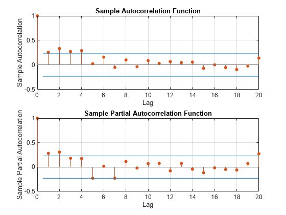
The sample ACF of the differenced series decays more quickly. The sample PACF cuts off after lag 2. This behavior is consistent with a second-degree autoregressive (AR(2)) model.

Specify and Estimate an ARIMA(2,1,0) Model

Specify, and then estimate, an ARIMA(2,1,0) model for the log quarterly Australian CPI. This model has one degree of nonseasonal differencing and two AR lags. By default, the innovation distribution is Gaussian with a constant variance.

Mdl = arima(2,1,0); EstMdl = estimate(Mdl,y);

ARIMA(2,1,0) Model (Gaussian Distribution): Value StandardError TStatistic PValue __________ _____________ __________ _________ Constant 0.010072 0.0032802 3.0707 0.0021356 AR{1} 0.21206 0.095428 2.2222 0.026271 AR{2} 0.33728 0.10378 3.2499 0.0011543 Variance 9.2302e-05 1.1112e-05 8.3066 9.849e-17

Both AR coefficients are significant at the 0.05 significance level.

Check Goodness of Fit

Infer the residuals from the fitted model. Check that the residuals are normally distributed and uncorrelated.

res = infer(EstMdl,y); figure subplot(2,2,1) plot(res./sqrt(EstMdl.Variance)) title('Standardized Residuals') subplot(2,2,2) qqplot(res) subplot(2,2,3) autocorr(res) subplot(2,2,4) parcorr(res) hvec = findall(gcf,'Type','axes'); set(hvec,'TitleFontSizeMultiplier',0.8,...'LabelFontSizeMultiplier',0.8);

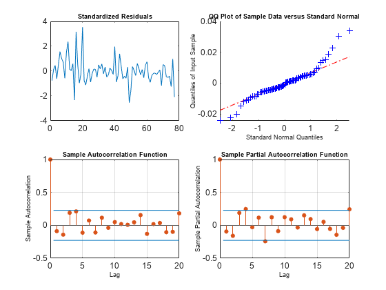
The residuals are reasonably normally distributed and uncorrelated.

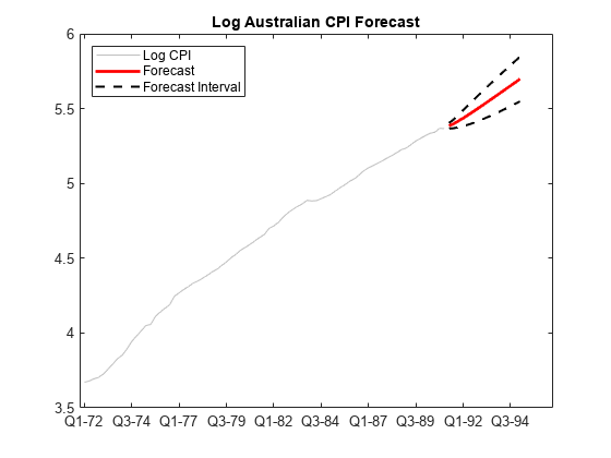
Generate Forecasts

Generate forecasts and approximate 95% forecast intervals for the next 4 years (16 quarters).

[yF,yMSE] = forecast(EstMdl,16,y); UB = yF + 1.96*sqrt(yMSE); LB = yF - 1.96*sqrt(yMSE); figure h4 = plot(y,'Color',[.75,.75,.75]); holdonh5 = plot(78:93,yF,'r','LineWidth',2); h6 = plot(78:93,UB,'k--','LineWidth',1.5); plot(78:93,LB,'k--','LineWidth',1.5); fDates = [dates; dates(T) + cumsum(diff(dates(T-16:T)))]; h7 = gca; h7.XTick = 1:10:(T+16); h7.XTickLabel = datestr(fDates(1:10:end),17); legend([h4,h5,h6],'Log CPI','Forecast',...'Forecast Interval','Location','Northwest') title('Log Australian CPI Forecast') holdoff

References:

Box, G. E. P., G. M. Jenkins, and G. C. Reinsel.Time Series Analysis: Forecasting and Control. 3rd ed. Englewood Cliffs, NJ: Prentice Hall, 1994.