柔性梁的模型

Figure 1 depicts an active vibration control system for a flexible beam.

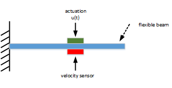
Figure 1: Active control of flexible beam

在此设置中，执行力的执行器和the velocity sensor are collocated. We can model the transfer function from control inputto the velocity使用有限元分析。仅保留前六个模式，我们获得了形式的植物模型

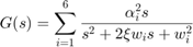
具有以下参数值。

％ 参数xi = 0.05;alpha = [0.09877，-0.309，-0.891，0.5878，0.7071，-0.8091];w = [1，4，9，16，25，36];

The resulting beam model foris given by

% Beam modelG = tf(alpha(1)^2*[1,0],[1, 2*xi*w(1), w(1)^2]) +。。。tf(alpha(2)^2*[1,0],[1, 2*xi*w(2), w(2)^2]) +。。。tf（alpha（3）^2*[1,0]，[1，2*xi*w（3），w（3）^2]） +。。。tf(alpha(4)^2*[1,0],[1, 2*xi*w(4), w(4)^2]) +。。。tf(alpha(5)^2*[1,0],[1, 2*xi*w(5), w(5)^2]) +。。。tf(alpha(6)^2*[1,0],[1, 2*xi*w(6), w(6)^2]); G.InputName ='uG';G.Outputname ='y';

使用此传感器/执行器配置，光束是一个被动系统：

ISAPPANSIVE（G）

ans =逻辑1

通过观察到这一点的奈奎斯特情节证实了这一点是正的真实。

nyquist(G)

LQG控制器

LQG控制是主动振动控制的自然公式。LQG控制设置如图2所示。信号和are the process and measurement noise, respectively.

Figure 2: LQG control structure

First useLQGto compute the optimal LQG controller for the objective

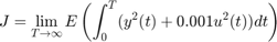
with noise variances:

[a,b,c,d] = ssdata(G); M = [c d;zeros(1,12) 1];% [y;u] = M * [x;u]QWV = blkdiag(b*b',1e-2); QXU = M'*diag([1 1e-3])*M; CLQG = lqg(ss(G),QXU,QWV);

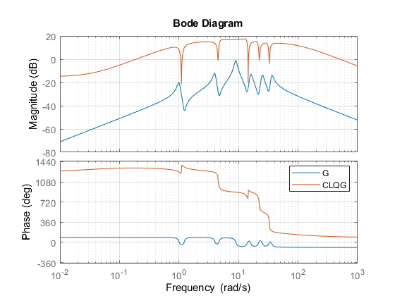
LQG-optimal控制器CLQGis complex with 12 states and several notching zeros.

size(CLQG)

State-space model with 1 outputs, 1 inputs, and 12 states.

bode(G,CLQG,{1e-2,1e3}), grid, legend('G','CLQG')

Use the general-purpose tunersystune尝试简化此控制器。和systune, you are not limited to a full-order controller and can tune controllers of any order. Here for example, let's tune a 2nd-order state-space controller.

c = ltiblock.ss（'C'、2、1,1);

Build a closed-loop model of the block diagram in Figure 2.

C.InputName ='yn';C.Outputname ='u';S1 = sumblk('yn = y + n'）；S2 = sumblk('ug = u + d'）；CL0 = connect(G,C,S1,S2,{'d','n'},{'y','u'},{'yn','u'});

使用LQG标准上面是唯一的调整目标。LQG调整目标使您可以直接指定性能权重和噪声协方差。

R1 = TuningGoal.LQG({'d','n'},{'y','u'}，diag（[1,1e-2]），diag（[1 1e-3]））;

现在调整控制器Cto minimize the LQG objective。

[CL1，J1] = Systune（CL0，R1）;

Final: Soft = 0.478, Hard = -Inf, Iterations = 40

优化器找到了一个二阶控制器。与最佳价值CLQG:

[〜，jopt] = evalgoal（r1，替换block（cl0，'C',CLQG))

Jopt = 0.4673

The performance degradation is less than 5%, and we reduced the controller complexity from 12 to 2 states. Further compare the impulse responses fromtofor the two controllers. The two responses are almost identical. You can therefore obtain near-optimal vibration attenuation with a simple second-order controller.

t0 =反馈（g，clqg，+1）;t1 = getiotransfer（cl1，'d','y'）；impulse(T0,T1,5) title('Response to impulse disturbance d') legend('LQG optimal','2nd-order LQG')

被动LQG控制器

我们使用横梁的近似模型来设计这两个控制器。先验，不能保证这些控制器在真实梁上的性能很好。但是，我们知道光束是一个被动物理系统，被动系统的负反馈互连始终是稳定的。因此，如果is passive, we can be confident that the closed-loop system will be stable.

The optimal LQG controller is not passive. In fact, its relative passive index is infinite because甚至不是最小阶段。

getPassiveIndex（-clqg）

ans = Inf

它的奈奎斯特情节证实了这一点。

nyquist(-CLQG)

Usingsystune，您可以重新调整二阶控制器，并以其他要求应该是被动的。为此，请从yntou(which is）。使用“加权可通过”目标来说明减号。

r2 = tuninggoal.WeightedPassitive（{'yn'},{'u'}，-1,1）;r2.openings ='u';

现在重新调整闭环模型CL1to minimize the LQG objectivesubject tobeing passive. Note that the passivity goalR2现在被指定为硬约束。

[CL2,J2,g] = systune(CL1,R1,R2);

Final: Soft = 0.478, Hard = 1, Iterations = 51

The tuner achieves the same如前所述，在执行被动性的同时（硬约束小于1）。验证这一点是被动的。

c2 = getBlockValue（cl2，'C'）；被动图（-c2）

The improvement over the LQG-optimal controller is most visible in the Nyquist plot.

nyquist(-CLQG,-C2) legend('LQG optimal','2nd-order passive LQG')

最后，比较来自to。

T2 = getIOTransfer(CL2,'d','y'）；impulse(T0,T2,5) title('Response to impulse disturbance d') legend('LQG optimal','2nd-order passive LQG')

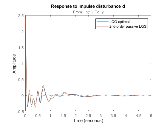
Usingsystune，您设计了一个二阶被动控制器，具有近乎最佳的LQG性能。