Online Recursive Least Squares Estimation
This example shows how to implement an online recursive least squares estimator. You estimate a nonlinear model of an internal combustion engine and use recursive least squares to detect changes in engine inertia.
Engine Model
The engine model includes nonlinear elements for the throttle and manifold system, and the combustion system. The model input is the throttle angle and the model output is the engine speed in rpm.
open_system('iddemo_engine'); sim('iddemo_engine')
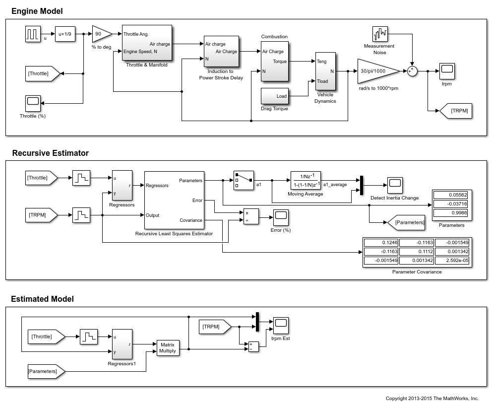
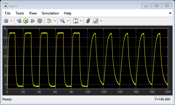
The engine model is set up with a pulse train driving the throttle angle from open to closed. The engine response is nonlinear, specifically the engine rpm response time when the throttle is open and closed are different.
At 100 seconds into the simulation an engine fault occurs causing the engine inertia to increase (the engine inertia,J, is modeled in theiddemo_engine/Vehicle Dynamicsblock). The inertia change causes engine response times at open and closed throttle positions to increase. You use online recursive least squares to detect the inertia change.
open_system('iddemo_engine/trpm')
Estimation Model
The engine model is a damped second order system with input and output nonlinearities to account for different response times at different throttle positions. Use the recursive least squares block to identify the following discrete system that models the engine:

Since the estimation model does not explicitly include inertia we expect the values to change as the inertia changes. We use the changingvalues to detect the inertia change.
The engine has significant bandwidth up to 16Hz. Set the estimator sampling frequency to 2*160Hz or a sample time of seconds.
Recursive Least Squares Estimator Block Setup
The terms in the estimated model are themodel regressorsand inputs to the recursive least squares block that estimates thevalues. You can implement the regressors as shown in the
iddemo_engine/Regressorsblock.
open_system('iddemo_engine/Regressors');

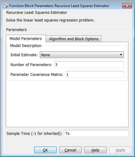
Configure the Recursive Least Squares Estimator block:
Initial Estimate:None. By default, the software uses a value of 1.
Number of parameters: 3, one for each
 regressor coefficient.
Parameter Covariance Matrix: 1, the amount of uncertainty in initial guess of 1. Concretely, treat the estimated parameters as a random variable with variance 1.
Sample Time:
 .
.

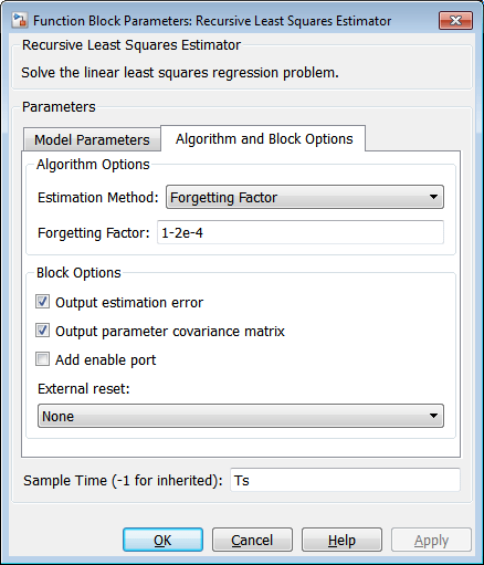
ClickAlgorithm and Block Optionsto set the estimation options:
Estimation Method:
Forgetting Factor
Forgetting Factor: 1-2e-4. Since the estimated
values are expected to change with the inertia, set the forgetting factor to a value less than 1. Choose = 1-2e-4 which corresponds to a memory time constant of
 or 15 seconds. A 15 second memory time ensures that significant data from both the open and closed throttle position are used for estimation as the position is changed every 10 seconds.


Select theOutput estimation errorcheck box. You use this block output to validate the estimation.
Select theOutput parameter covariance matrixcheck box. You use this block output to validate the estimation.
Clear theAdd enable portcheck box.
External reset:
None.
Validating the Estimated Model
TheErroroutput of theRecursive Least Squares Estimator块给estim领先一步的错误ated model. This error is less than 5% indicating that for one-step-ahead prediction the estimated model is accurate.
open_system('iddemo_engine/Error (%)')

The diagonal of the parameter covariances matrix gives the variances for the parameters. The
 variance is small relative to the parameter value indicating good confidence in the estimated value. In contrast, the
 variances are large relative to the parameter values indicating a low confidence in these values.

While the small estimation error and covariances give confidence that the model is being estimated correctly, it is limited in that the error is a one-step-ahead predictor. A more rigorous check is to use the estimated model in a simulation model and compare with the actual model output. TheEstimated Modelsection of the simulink model implements this.
TheRegressors1block is identical to theRegressors块使用递归估计量。唯一difference is that the y signal is not measured from the plant but fed back from the output of the estimated model. The Output of the regressors block is multiplied by estimatedvalues to give an estimate of the engine speed.
open_system('iddemo_engine/trpm Est')
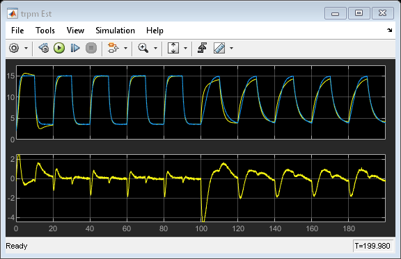
The estimated model output matches the model output fairly well. The steady-state values are close and the transient behavior is slightly different but not significantly so. Note that after 100 seconds when the engine inertia changes the estimated model output differs slightly more from the model output. This implies that the chosen regressors cannot capture the behavior of the model as well after the inertia change. This also suggests a change in system behavior.
The estimated model output combined with the low one-step-ahead error and parameter covariances gives us confidence in the recursive estimator.
Detecting Changes in Engine Inertia
The engine model is setup to introduce an inertia change 100 seconds into the simulation. The recursive estimator can be used to detect the change in inertia.
The recursive estimator takes around 50 seconds to converge to an initial set of parameter values. To detect the inertia change we examine the model coefficient that influences the
 term of the estimated model.
open_system('iddemo_engine/Detect Inertia Change')

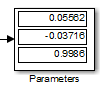
The covariance for, 0.05562, is large relative to the parameter value 0.1246 indicating low confidence in the estimated value. The time plot ofshows why the covariance is large. Specificallyis varying as the throttle position varies indicating that the estimated model is not rich enough to fully capture different rise times at different throttle positions and needs to adjust. However, we can use this to identify the inertia changes as the average value ofchanges as the inertia changes. You can use a threshold detector on the moving average of theparameter to detect changes in the engine inertia.
bdclose('iddemo_engine')
You can also select a web site from the following list:
Americas
- América Latina(Español)
- Canada(English)
- United States(English)
Europe
- Belgium(English)
- Denmark(English)
- Deutschland(Deutsch)
- España(Español)
- Finland(English)
- France(Français)
- Ireland(English)
- Italia(Italiano)
- Luxembourg(English)
- Netherlands(English)
- Norway(English)
- Österreich(Deutsch)
- Portugal(English)
- Sweden(English)
- Switzerland
- United Kingdom(English)