Derive and Apply Inverse Kinematics to Two-Link Robot Arm

打开实时脚本

该示例通过使用MATLAB®和Symbolic Math Toolbox™来推导并将逆运动学应用于两连锁机器人组。

该示例象征性地定义了关节参数和最终效应器位置，计算和可视化运动和逆运动溶液，并找到系统jacobian，这对于模拟机器人组的运动很有用。万博尤文图斯

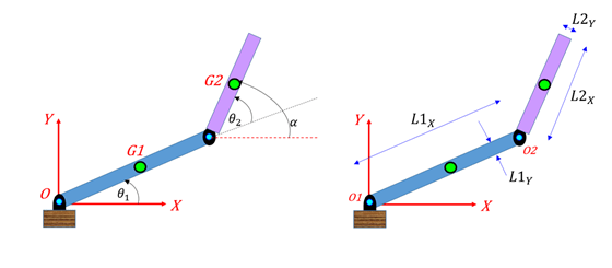
Step 1: Define Geometric Parameters

将机器人的链路长度，关节角度和最终效应器位置定义为符号变量。

symsL_1L_2theta_1theta_2XEYE

指定机器人链路长度的值。

L1 = 1;L2 = 0.5;

Step 2: Define X and Y Coordinates of End Effector

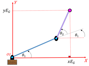
定义最终效应器的X和Y坐标作为关节角度的函数 $(θ_{1}, θ_{2})$ 。

XE_RHS = l_1*cos（theta_1） + l_2*cos（theta_1 + theta_2）

XE_RHS =
                   $L_{2} \cos (θ_{1} + θ_{2}) + L_{1} \cos (θ_{1})$

YE_RHS = L_1*sin(theta_1) + L_2*sin(theta_1+theta_2)

YE_RHS =
                   $L_{2} \sin (θ_{1} + θ_{2}) + L_{1} \sin (θ_{1})$

Convert the symbolic expressions into MATLAB functions.

XE_MLF = matlabFunction(XE_RHS,'Vars',[L_1 L_2 theta_1 theta_2]); YE_MLF = matlabFunction(YE_RHS,'Vars',[L_1 L_2 theta_1 theta_2]);

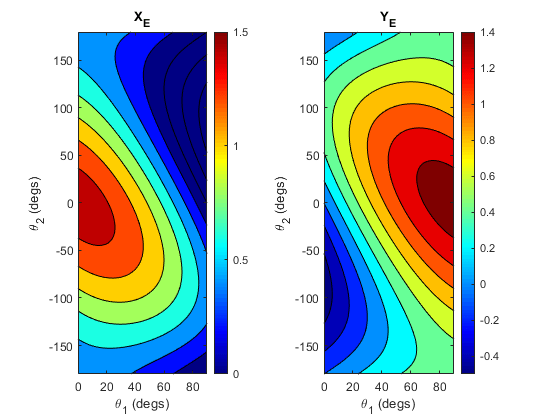
Step 3: Calculate and Visualize Forward Kinematics

向前运动学将关节角度转化为最终效应的位置： $(θ_{1}, θ_{2}) ⟶ f (θ_{1}, θ_{2}) ⟶ (X_{E}, Y_{E})$ 。Given specific joint-angle values, use forward kinematics to calculate the end-effector locations.

将关节角的输入值指定为 $0^{\circ} < θ_{1} < 90^{\circ}$ 和 ${- 180}^{\circ} < θ_{2} < 180^{\circ}$ 。

t1_degs_row = linspace（0,90,100）;t2_degs_row = linspace（-180,180,100）;[tt1_degs，tt2_degs] = meshgrid（t1_degs_row，t2_degs_row）;

Convert the angle units from degrees to radians.

tt1_rads = deg2rad(tt1_degs); tt2_rads = deg2rad(tt2_degs);

Calculate the X and Y coordinates using the MATLAB functionsXE_MLF和YE_MLF, respectively.

X_mat = XE_MLF(L1,L2,tt1_rads,tt2_rads); Y_mat = YE_MLF(L1,L2,tt1_rads,tt2_rads);

使用辅助功能可视化X和Y坐标plot_xy_given_theta_2dof。

plot_xy_given_theta_2dof（tt1_degs，tt2_degs，x_mat，y_mat，（l1+l2））

图包含2个轴对象。轴对象1带标题x索引的基线包含类型轮廓的对象。轴对象2带标题y索引的基线包含类型轮廓的对象。

Step 4:查找逆运动学

Inverse kinematics transforms the end-effector locations into joint angles: $(X_{E}, Y_{E}) ⟶ g (X_{E}, Y_{E}) ⟶ (θ_{1}, θ_{2})$ 。从正向运动学方程式找到逆运动学。

Define the forward kinematics equations.

XE_EQ = XE == XE_RHS; YE_EQ = YE == YE_RHS;

解决 $θ_{1}$ 和 $θ_{2}$ 。

s =solve([XE_EQ YE_EQ], [theta_1 theta_2])

s =带有字段的结构：theta_1: [2x1 sym] theta_2: [2x1 sym]

结构S代表多个解决方案万博尤文图斯 $θ_{1}$ 和 $θ_{2}$ 。Show the pair of solutions for $θ_{1}$ 。

简化（s.theta_1）

ans =
                  
                    $\begin{array}{l} (\begin{array}{c} 2 晒黑 (\frac{2 L_{1} YE + σ_{1}}{{L_{1}}^{2} + 2 L_{1} XE - {L_{2}}^{2} + {XE}^{2} + {YE}^{2}}) \\ 2 晒黑 (\frac{2 L_{1} YE - σ_{1}}{{L_{1}}^{2} + 2 L_{1} XE - {L_{2}}^{2} + {XE}^{2} + {YE}^{2}}) \end{array}) \\ where \\ σ_{1} = \sqrt{- {L_{1}}^{4} + 2 {L_{1}}^{2} {L_{2}}^{2} + 2 {L_{1}}^{2} {XE}^{2} + 2 {L_{1}}^{2} {YE}^{2} - {L_{2}}^{4} + 2 {L_{2}}^{2} {XE}^{2} + 2 {L_{2}}^{2} {YE}^{2} - {XE}^{4} - 2 {XE}^{2} {YE}^{2} - {YE}^{4}} \end{array}$

Show the pair of solutions for $θ_{2}$ 。

简化（s.theta_2）

ans =
                  
                    $\begin{array}{l} (\begin{array}{c} - σ_{1} \\ σ_{1} \end{array}) \\ where \\ σ_{1} = 2 晒黑 (\frac{\sqrt{(- {L_{1}}^{2} + 2 L_{1} L_{2} - {L_{2}}^{2} + {XE}^{2} + {YE}^{2}) ({L_{1}}^{2} + 2 L_{1} L_{2} + {L_{2}}^{2} - {XE}^{2} - {YE}^{2})}}{- {L_{1}}^{2} + 2 L_{1} L_{2} - {L_{2}}^{2} + {XE}^{2} + {YE}^{2}}) \end{array}$

Convert the solutions into MATLAB functions that you can use later. The functionsTH1_MLF和TH2_MLF代表逆运动学。

TH1_MLF{1} = matlabFunction(S.theta_1(1),'Vars'，[l_1 l_2 xe ye]）;th1_mlf {2} = matlabFunction（s.theta_1（2），'Vars'，[l_1 l_2 xe ye]）;th2_mlf {1} = matlabFunction（s.theta_2（1），'Vars'，[l_1 l_2 xe ye]）;th2_mlf {2} = matlabFunction（s.theta_2（2），，'Vars'，[l_1 l_2 xe ye]）;

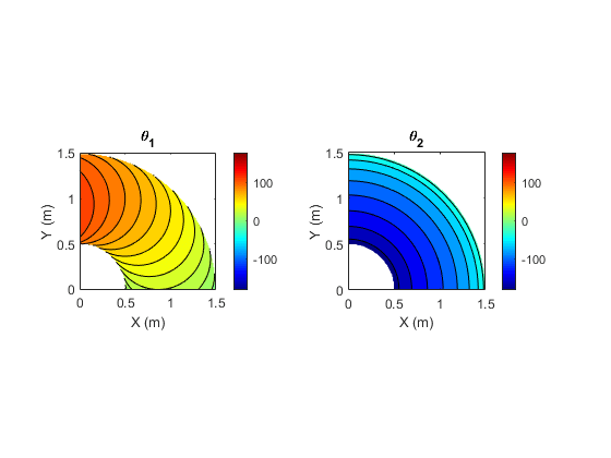
步骤5：计算和可视化逆运动学

Use the inverse kinematics to compute $θ_{1}$ 和 $θ_{2}$ from the X and Y coordinates.

定义X和Y坐标的网格点。

[xmat,ymat] = meshgrid(0:0.01:1.5,0:0.01:1.5);

Calculate the angles $θ_{1}$ 和 $θ_{2}$ 使用MATLAB功能sTH1_MLF{1}和th2_mlf {1}, respectively.

tmp_th1_mat = TH1_MLF{1}(L1,L2,xmat,ymat); tmp_th2_mat = TH2_MLF{1}(L1,L2,xmat,ymat);

Convert the angle units from radians to degrees.

tmp_th1_mat = rad2deg(tmp_th1_mat); tmp_th2_mat = rad2deg(tmp_th2_mat);

Some of the input coordinates, such as (X,Y) = (1.5,1.5), are beyond the reachable workspace of the end effector. The inverse kinematics solutions can generate some imaginary theta values that require correction. Correct the imaginary theta values.

th1_mat = NaN(size(tmp_th1_mat)); th2_mat = NaN(size(tmp_th2_mat)); tf_mat = imag(tmp_th1_mat) == 0; th1_mat(tf_mat) = real(tmp_th1_mat(tf_mat)); tf_mat = imag(tmp_th2_mat) == 0; th2_mat(tf_mat) = real(tmp_th2_mat(tf_mat));

Visualize the angles $θ_{1}$ 和 $θ_{2}$ using the helper functionplot_theta_given_XY_2dof。

plot_theta_given_XY_2dof(xmat,ymat,th1_mat,th2_mat)

图包含2个轴对象。Axes object 1 with title theta indexOf 1 baseline contains an object of type contour. Axes object 2 with title theta indexOf 2 baseline contains an object of type contour.

Step 6: Compute System Jacobian

系统的定义雅各比式是：

$J = \frac{d (X, Y)}{d (θ_{1}, θ_{2})} = (\begin{array}{c} \frac{d X}{d θ_{1}} & \frac{d X}{d θ_{2}} \\ \frac{d Y}{d θ_{1}} & \frac{d Y}{d θ_{2}} \end{array})$

the_j = jacobian（[xe_rhs ye_rhs]，[theta_1 theta_2]）

the_J =
                  
                    $(\begin{array}{c} - L_{2} \sin (θ_{1} + θ_{2}) - L_{1} \sin (θ_{1}) & - L_{2} \sin (θ_{1} + θ_{2}) \\ L_{2} \cos (θ_{1} + θ_{2}) + L_{1} \cos (θ_{1}) & L_{2} \cos (θ_{1} + θ_{2}) \end{array})$

您可以通过使用系统Jacobian将联合速度与最终效应速度相关联，而另一方面的方式将关节速度联系起来：

MATLAB $(\begin{array}{c} \frac{d X}{d t} \\ \frac{d Y}{d t} \end{array}) = (\begin{array}{c} \frac{d X}{d θ_{1}} & \frac{d X}{d θ_{2}} \\ \frac{d Y}{d θ_{1}} & \frac{d Y}{d θ_{2}} \end{array}) 。 (\begin{array}{c} \frac{d θ_{1}}{d t} \\ \frac{d θ_{2}}{d t} \end{array})$

$(\begin{array}{c} \frac{d X}{d t} \\ \frac{d Y}{d t} \end{array}) = J 。 (\begin{array}{c} \frac{d θ_{1}}{d t} \\ \frac{d θ_{2}}{d t} \end{array})$

$(\begin{array}{c} \frac{d θ_{1}}{d t} \\ \frac{d θ_{2}}{d t} \end{array}) = J^{+} 。 (\begin{array}{c} \frac{d X}{d t} \\ \frac{d Y}{d t} \end{array}) w h e r e J^{+} 是 the 摩尔 - 彭罗斯伪为的 J$

您还可以将雅各布的符号表达式转换为MATLAB功能块。通过将多个路点定义为simulink®模型的输入，模拟机器人在轨迹上的最终效应器位置。万博1manbetxSimu万博1manbetxlink模型可以根据关节角度值计算运动核心，以达到轨迹中的每个路点。有关更多详细信息，请参阅2链接机器人臂的逆运动学和教僵硬的身体动态。

Helper Functions

功能plot_theta_given_XY_2dof(X_mat,Y_mat,theta_1_mat_degs,。。。theta_2_mat_degs）xlab_str ='x（m）';ylab_str ='y（m）';数字;hax（1）=子图（1,2,1）;contourf(X_mat, Y_mat, theta_1_mat_degs); caxis(hax(1), [-180 180]); colormap(gca,'jet'); colorbar xlabel(xlab_str,“口译员”,'Tex'); ylabel(ylab_str,“口译员”,'Tex'); title(hax(1),'\ theta_1',“口译员”,'Tex') axis('平等的') hax(2) = subplot(1,2,2); contourf(X_mat, Y_mat, theta_2_mat_degs); caxis(hax(2), [-180 180]); colormap(gca,'jet'); colorbar xlabel(xlab_str,“口译员”,'Tex'); ylabel(ylab_str,“口译员”,'Tex'); title(hax(2),'\ theta_2',“口译员”,'Tex') axis('平等的')end功能plot_xy_given_theta_2dof(theta_1_mat_degs,theta_2_mat_degs,。。。x_mat，y_mat，a_cmax）xlab_str ='\ theta_1（degs）';ylab_str ='\theta_2 (degs)';数字;hax（1）=子图（1,2,1）;CONTOURF（theta_1_mat_degs，theta_2_mat_degs，x_mat）;Caxis（hax（1），[0 a_cmax]）;colormap（GCA，'jet'); colorbar xlabel(xlab_str,“口译员”,'Tex'); ylabel(ylab_str,“口译员”,'Tex'); title(hax(1),'X_E',“口译员”,'Tex') hax(2) = subplot(1,2,2); contourf(theta_1_mat_degs, theta_2_mat_degs, Y_mat); caxis(hax(1), [0 a_cmax]); colormap(gca,'jet'); colorbar xlabel(xlab_str,“口译员”,'Tex'); ylabel(ylab_str,“口译员”,'Tex'); title(hax(2),'Y_E',“口译员”,'Tex')end