Train Generalized Additive Model for Binary Classification

Load Sample Data

Load the 1994 census data stored incensus1994.mat. The data set consists of demographic data from the US Census Bureau to predict whether an individual makes over $50,000 per year. The classification task is to fit a model that predicts the salary category of people given their age, working class, education level, marital status, race, and so on.

loadcensus1994

census1994contains the training data setadultdataand the test data setadulttest. To reduce the running time for this example, subsample 500 training observations and 500 test observations by using thedatasample函数。

rng(1)% For reproducibilityNumSamples = 5e2; adultdata = datasample(adultdata,NumSamples,'Replace',false); adulttest = datasample(adulttest,NumSamples,'Replace',false);

Train GAM with Optimal Hyperparameters

Train a GAM with hyperparameters that minimize the cross-validation loss by using theOptimizeHyperparametersname-value argument.

You can specifyOptimizeHyperparametersas'auto'or'all'to find optimal hyperparameter values for both univariate and bivariate parameters. Alternatively, you can find optimal values for univariate parameters using the'auto-univariate'or'all-univariate'option, and then find optimal values for bivariate parameters using the'auto-bivariate'or'all-bivariate'option. This example uses'auto-univariate'and'auto-bivariate'.

Train a univariate GAM. SpecifyOptimizeHyperparametersas'auto-univariate'so thatfitcgamfinds optimal values of theInitialLearnRateForPredictorsandNumTreesPerPredictorname-value arguments. For reproducibility, use the'expected-improvement-plus'acquisition function. SpecifyShowPlotsasfalseandVerboseas 0 to disable plot and message displays, respectively.

Mdl_univariate = fitcgam(adultdata,'salary','Weights','fnlwgt',...'OptimizeHyperparameters','auto-univariate',...'HyperparameterOptimizationOptions',struct('AcquisitionFunctionName','expected-improvement-plus',...'ShowPlots',false,'Verbose',0))

Mdl_univariate = ClassificationGAM PredictorNames: {'age' 'workClass' 'education' 'education_num' 'marital_status' 'occupation' 'relationship' 'race' 'sex' 'capital_gain' 'capital_loss' 'hours_per_week' 'native_country'} ResponseName: 'salary' CategoricalPredictors: [2 3 5 6 7 8 9 13] ClassNames: [<=50K >50K] ScoreTransform: 'logit' Intercept: -1.3118 NumObservations: 500 HyperparameterOptimizationResults: [1×1 BayesianOptimization] Properties, Methods

fitcgam返回一个ClassificationGAMmodel object that uses the best estimated feasible point. The best estimated feasible point indicates the set of hyperparameters that minimizes the upper confidence bound of the objective function value based on the underlying objective function model of the Bayesian optimization process. You can obtain the best point from theHyperparameterOptimizationResultsproperty or by using thebestPoint函数。

x = Mdl_univariate.HyperparameterOptimizationResults.XAtMinEstimatedObjective

x=1×2 tableInitialLearnRateForPredictors NumTreesPerPredictor _____________________________ ____________________ 0.02257 118

bestPoint(Mdl_univariate.HyperparameterOptimizationResults)

ans=1×2 tableInitialLearnRateForPredictors NumTreesPerPredictor _____________________________ ____________________ 0.02257 118

For more details on the optimization process, seeOptimize GAM Using OptimizeHyperparameters.

Train a bivariate GAM. SpecifyOptimizeHyperparametersas'auto-bivariate'so thatfitcgamfinds optimal values of theInteractions,InitialLearnRateForInteractions, andNumTreesPerInteractionname-value arguments. Use the univariate parameter values inxso that the software finds optimal parameter values for interaction terms based on the x values.

Mdl = fitcgam(adultdata,'salary','Weights','fnlwgt',...'InitialLearnRateForPredictors',x.InitialLearnRateForPredictors,...'NumTreesPerPredictor',x.NumTreesPerPredictor,...'OptimizeHyperparameters','auto-bivariate',...'HyperparameterOptimizationOptions',struct('AcquisitionFunctionName','expected-improvement-plus',...'ShowPlots',false,'Verbose',0))

Mdl = ClassificationGAM PredictorNames: {'age' 'workClass' 'education' 'education_num' 'marital_status' 'occupation' 'relationship' 'race' 'sex' 'capital_gain' 'capital_loss' 'hours_per_week' 'native_country'} ResponseName: 'salary' CategoricalPredictors: [2 3 5 6 7 8 9 13] ClassNames: [<=50K >50K] ScoreTransform: 'logit' Intercept: -1.4587 Interactions: [6×2 double] NumObservations: 500 HyperparameterOptimizationResults: [1×1 BayesianOptimization] Properties, Methods

Display the optimal bivariate hyperparameters.

Mdl.HyperparameterOptimizationResults.XAtMinEstimatedObjective

ans=1×3 tableInteractions InitialLearnRateForInteractions NumTreesPerInteraction ____________ _______________________________ ______________________ 6 0.0061954 422

The model display ofMdlshows a partial list of the model properties. To view the full list of the model properties, double-click the variable nameMdlin the Workspace. The Variables editor opens forMdl. Alternatively, you can display the properties in the Command Window by using dot notation. For example, display theReasonForTerminationproperty.

Mdl.ReasonForTermination

ans =struct with fields:PredictorTrees: 'Terminated after training the requested number of trees.' InteractionTrees: 'Terminated after training the requested number of trees.'

You can use theReasonForTerminationproperty to determine whether the trained model contains the specified number of trees for each linear term and each interaction term.

Display the interaction terms inMdl.

Mdl.Interactions

ans =6×25 12 1 6 6 12 1 12 7 9 2 6

Each row ofInteractionsrepresents one interaction term and contains the column indexes of the predictor variables for the interaction term. You can use theInteractionsproperty to check the interaction terms in the model and the order in whichfitcgamadds them to the model.

Display the interaction terms inMdlusing the predictor names.

Mdl.PredictorNames(Mdl.Interactions)

ans =6×2 cell{'marital_status'} {'hours_per_week'} {'age' } {'occupation' } {'occupation' } {'hours_per_week'} {'age' } {'hours_per_week'} {'relationship' } {'sex' } {'workClass' } {'occupation' }

Assess Predictive Performance on New Observations

Assess the performance of the trained model by using the test sampleadulttestand the object functionspredict,loss,edge, andmargin. You can use a full or compact model with these functions.

If you want to assess the performance of the training data set, use the resubstitution object functions:resubPredict,resubLoss,resubMargin, andresubEdge. To use these functions, you must use the full model that contains the training data.

Create a compact model to reduce the size of the trained model.

CMdl = compact(Mdl); whos('Mdl','CMdl')

Name Size Bytes Class Attributes CMdl 1x1 5126918 classreg.learning.classif.CompactClassificationGAM Mdl 1x1 5272831 ClassificationGAM

Predict labels and scores for the test data set (adulttest), and compute model statistics (loss, margin, and edge) using the test data set.

[labels,scores] = predict(CMdl,adulttest); L = loss(CMdl,adulttest,'Weights',adulttest.fnlwgt); M = margin(CMdl,adulttest); E = edge(CMdl,adulttest,'Weights',adulttest.fnlwgt);

Predict labels and scores and compute the statistics without including interaction terms in the trained model.

[labels_nointeraction,scores_nointeraction] = predict(CMdl,adulttest,'IncludeInteractions',false); L_nointeractions = loss(CMdl,adulttest,'Weights',adulttest.fnlwgt,'IncludeInteractions',false); M_nointeractions = margin(CMdl,adulttest,'IncludeInteractions',false); E_nointeractions = edge(CMdl,adulttest,'Weights',adulttest.fnlwgt,'IncludeInteractions',false);

Compare the results obtained by including both linear and interaction terms to the results obtained by including only linear terms.

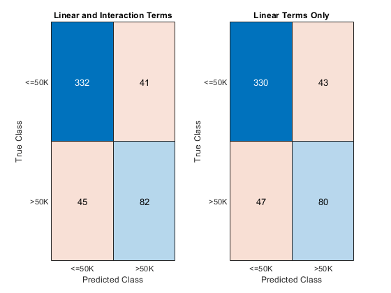
Create a confusion chart from the true labelsadulttest.salaryand the predicted labels.

tiledlayout(1,2); nexttile confusionchart(adulttest.salary,labels) title('Linear and Interaction Terms') nexttile confusionchart(adulttest.salary,labels_nointeraction) title('Linear Terms Only')

Display the computed loss and edge values.

table([L; E], [L_nointeractions; E_nointeractions],...'VariableNames',{'Linear and Interaction Terms','Only Linear Terms'},...'RowNames',{'Loss','Edge'})

ans=2×2 tableLinear and Interaction Terms Only Linear Terms ____________________________ _________________ Loss 0.1748 0.17872 Edge 0.57902 0.54756

The model achieves a smaller loss value and a higher edge value when both linear and interaction terms are included.

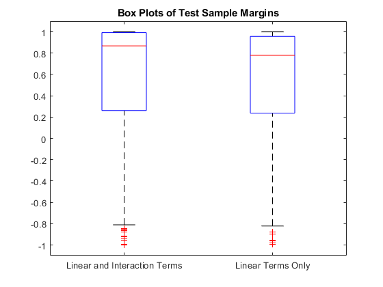
Display the distributions of the margins using box plots.

figure boxplot([M M_nointeractions],'Labels',{'Linear and Interaction Terms','Linear Terms Only'}) title('Box Plots of Test Sample Margins')

Interpret Prediction

Interpret the prediction for the first test observation by using theplotLocalEffects函数。Also, create partial dependence plots for some important terms in the model by using theplotPartialDependence函数。

Classify the first observation of the test data, and plot the local effects of the terms inCMdlon the prediction. To display an existing underscore in any predictor name, change theTickLabelInterpretervalue of the axes to'none'.

[label,score] = predict(CMdl,adulttest(1,:))

label =categorical<=50K

score =1×20.9895 0.0105

f1 = figure; plotLocalEffects(CMdl,adulttest(1,:)) f1.CurrentAxes.TickLabelInterpreter ='none';

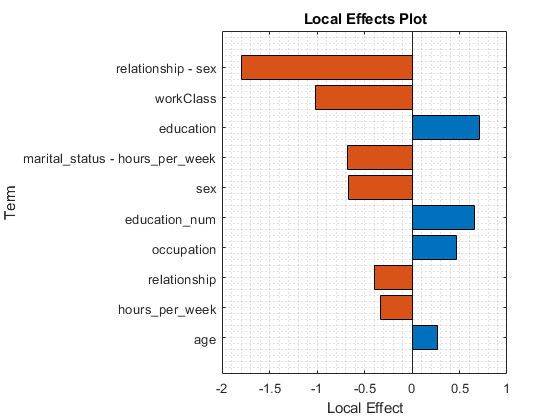
Thepredict函数将第一次观察到adulttest(1,:)as'<=50K'. TheplotLocalEffectsfunction creates a horizontal bar graph that shows the local effects of the 10 most important terms on the prediction. Each local effect value shows the contribution of each term to the classification score for'<=50K', which is the logit of the posterior probability that the classification is'<=50K'for the observation.

Create a partial dependence plot for the termage. Specify both the training and test data sets to compute the partial dependence values using both sets.

figure plotPartialDependence(CMdl,'age',label,[adultdata; adulttest])

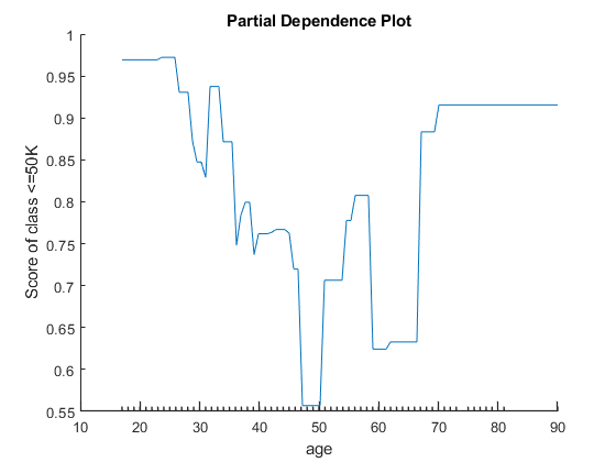
pl的otted line represents the averaged partial relationships between the predictorageand the score of the class<=50Kin the trained model. Thex-axis minor ticks represent the unique values in the predictorage.

Create partial dependence plots for the termseducation_numandrelationship.

f2 = figure; plotPartialDependence(CMdl,["education_num",“关系nship"],label,[adultdata; adulttest]) f2.CurrentAxes.TickLabelInterpreter ='none'; view([55 40])

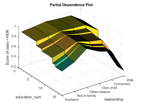
pl的ot shows the partial dependence of the score value for the class<=50oneducation_numandrelationship.