Specify Conditional Variance Model for Exchange Rates

Load the Data.

Load the exchange rate data included with the toolbox.

loadData_MarkPoundy = Data; T = length(y); figure plot(y) h = gca; h.XTick = [1 659 1318 1975]; h.XTickLabel = {＇Jan 1984',＇Jan 1986',＇Jan 1988',...＇Jan 1992'}; ylabel＇Exchange Rate'; title＇Deutschmark/British Pound Foreign Exchange Rate';

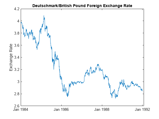
The exchange rate looks nonstationary (it does not appear to fluctuate around a fixed level).

Calculate the Returns.

Convert the series to returns. This results in the loss of the first observation.

r = price2ret(y); figure plot(2:T,r) h2 = gca; h2.XTick = [1 659 1318 1975]; h2.XTickLabel = {＇Jan 1984',＇Jan 1986',＇Jan 1988',...＇Jan 1992'}; ylabel＇Returns'; title“马克/英镑每日回报s';

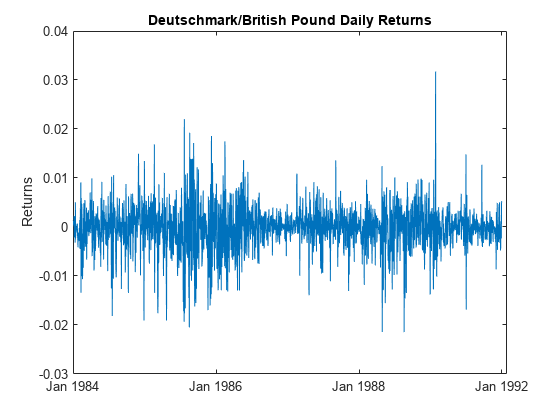
The returns series fluctuates around a common level, but exhibits volatility clustering. Large changes in the returns tend to cluster together, and small changes tend to cluster together. That is, the series exhibits conditional heteroscedasticity.

The returns are of relatively high frequency. Therefore, the daily changes can be small. For numerical stability, it is good practice to scale such data. In this case, scale the returns to percentage returns.

r = 100*r;

Check for Autocorrelation.

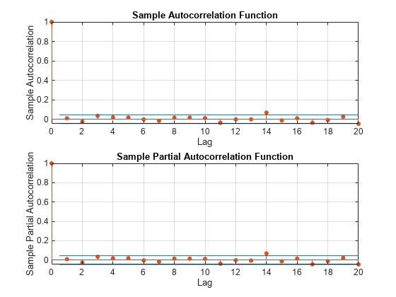
Check the returns series for autocorrelation. Plot the sample ACF and PACF, and conduct a Ljung-Box Q-test.

figure subplot(2,1,1) autocorr(r) subplot(2,1,2) parcorr(r)

[h,p] = lbqtest(r,＇Lags',[5 10 15])

h =1x3 logical array0 0 0

p =1×30.3982 0.7278 0.2109

The sample ACF and PACF show virtually no significant autocorrelation. The Ljung-Box Q-test null hypothesis that all autocorrelations up to the tested lags are zero is not rejected for tests at lags 5, 10, and 15. This suggests that a conditional mean model is not needed for this returns series.

Check for Conditional Heteroscedasticity.

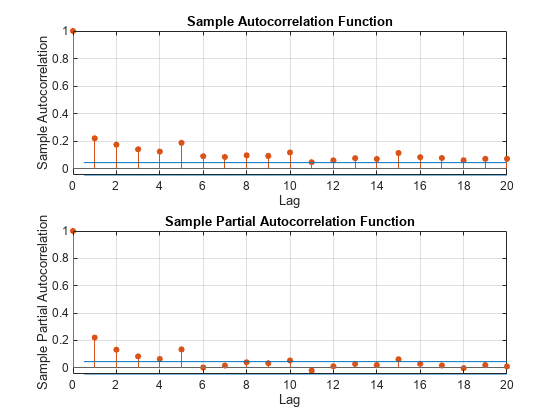
Check the return series for conditional heteroscedasticity. Plot the sample ACF and PACF of the squared returns series (after centering). Conduct Engle's ARCH test with a two-lag ARCH model alternative.

figure subplot(2,1,1) autocorr((r-mean(r)).^2) subplot(2,1,2) parcorr((r-mean(r)).^2)

[h,p] = archtest(r-mean(r),＇Lags',2)

h =logical1

p = 0

The sample ACF and PACF of the squared returns show significant autocorrelation. This suggests a GARCH model with lagged variances and lagged squared innovations might be appropriate for modeling this series. Engle's ARCH test rejects the null hypothesis (h = 1) of no ARCH effects in favor of the alternative ARCH model with two lagged squared innovations. An ARCH model with two lagged innovations is locally equivalent to a GARCH(1,1) model.

Specify a GARCH(1,1) Model.

Based on the autocorrelation and conditional heteroscedasticity specification testing, specify the GARCH(1,1) model with a mean offset:

with $${\epsilon }_t={\sigma }_t{z}_t$$and

Assume a Gaussian innovation distribution.

Mdl = garch(＇Offset',NaN,＇GARCHLags',1,＇ARCHLags',1)

Mdl = garch with properties: Description: "GARCH(1,1) Conditional Variance Model with Offset (Gaussian Distribution)" SeriesName: "Y" Distribution: Name = "Gaussian" P: 1 Q: 1 Constant: NaN GARCH: {NaN} at lag [1] ARCH: {NaN} at lag [1] Offset: NaN

The created model,Mdl, hasNaNvalues for all unknown parameters in the specified GARCH(1,1) model.

You can pass the GARCH modelMdlandrintoestimateto estimate the parameters.