Train Network with Numeric Features

Open Live Script

This example shows how to create and train a simple neural network for deep learning feature data classification.

If you have a data set of numeric features (for example a collection of numeric data without spatial or time dimensions), then you can train a deep learning network using a feature input layer. For an example showing how to train a network for image classification, seeCreate Simple Deep Learning Neural Network for Classification.

This example shows how to train a network to classify the gear tooth condition of a transmission system given a mixture of numeric sensor readings, statistics, and categorical labels.

Load Data

Load the transmission casing dataset for training. The data set consists of 208 synthetic readings of a transmission system consisting of 18 numeric readings and three categorical labels:

SigMean— Vibration signal mean
SigMedian— Vibration signal median
SigRMS— Vibration signal RMS
SigVar— Vibration signal variance
SigPeak— Vibration signal peak
SigPeak2Peak— Vibration signal peak to peak
SigSkewness— Vibration signal skewness
SigKurtosis— Vibration signal kurtosis
SigCrestFactor— Vibration signal crest factor
SigMAD— Vibration signal MAD
SigRangeCumSum— Vibration signal range cumulative sum
SigCorrDimension— Vibration signal correlation dimension
SigApproxEntropy— Vibration signal approximate entropy
SigLyapExponent— Vibration signal Lyap exponent
PeakFreq— Peak frequency.
HighFreqPower— High frequency power
EnvPower— Environment power
PeakSpecKurtosis— Peak frequency of spectral kurtosis
SensorCondition— Condition of sensor, specified as "Sensor Drift" or "No Sensor Drift"
ShaftCondition— Condition of shaft, specified as "Shaft Wear" or "No Shaft Wear"
GearToothCondition— Condition of gear teeth, specified as "Tooth Fault" or "No Tooth Fault"

Read the transmission casing data from the CSV file"transmissionCasingData.csv".

filename ="transmissionCasingData.csv"; tbl = readtable(filename,'TextType','String');

Convert the labels for prediction to categorical using theconvertvarsfunction.

labelName ="GearToothCondition"; tbl = convertvars(tbl,labelName,'categorical');

View the first few rows of the table.

head(tbl)

SigMean SigMedian SigRMS SigVar SigPeak SigPeak2Peak SigSkewness SigKurtosis SigCrestFactor SigMAD SigRangeCumSum SigCorrDimension SigApproxEntropy SigLyapExponent PeakFreq HighFreqPower EnvPower PeakSpecKurtosis SensorCondition ShaftCondition GearToothCondition ________ _________ ______ _______ _______ ____________ ___________ ___________ ______________ _______ ______________ ________________ ________________ _______________ ________ _____________ ________ ________________ _______________ _______________ __________________ -0.94876 -0.9722 1.3726 0.98387 0.81571 3.6314 -0.041525 2.2666 2.0514 0.8081 28562 1.1429 0.031581 79.931 0 6.75e-06 3.23e-07 162.13 "Sensor Drift" "No Shaft Wear" No Tooth Fault -0.97537 -0.98958 1.3937 0.99105 0.81571 3.6314 -0.023777 2.2598 2.0203 0.81017 29418 1.1362 0.037835 70.325 0 5.08e-08 9.16e-08 226.12 "Sensor Drift" "No Shaft Wear" No Tooth Fault 1.0502 1.0267 1.4449 0.98491 2.8157 3.6314 -0.04162 2.2658 1.9487 0.80853 31710 1.1479 0.031565 125.19 0 6.74e-06 2.85e-07 162.13 "Sensor Drift" "Shaft Wear" No Tooth Fault 1.0227 1.0045 1.4288 0.99553 2.8157 3.6314 -0.016356 2.2483 1.9707 0.81324 30984 1.1472 0.032088 112.5 0 4.99e-06 2.4e-07 162.13 "Sensor Drift" "Shaft Wear" No Tooth Fault 1.0123 1.0024 1.4202 0.99233 2.8157 3.6314 -0.014701 2.2542 1.9826 0.81156 30661 1.1469 0.03287 108.86 0 3.62e-06 2.28e-07 230.39 "Sensor Drift" "Shaft Wear" No Tooth Fault 1.0275 1.0102 1.4338 1.0001 2.8157 3.6314 -0.02659 2.2439 1.9638 0.81589 31102 1.0985 0.033427 64.576 0 2.55e-06 1.65e-07 230.39 "Sensor Drift" "Shaft Wear" No Tooth Fault 1.0464 1.0275 1.4477 1.0011 2.8157 3.6314 -0.042849 2.2455 1.9449 0.81595 31665 1.1417 0.034159 98.838 0 1.73e-06 1.55e-07 230.39 "Sensor Drift" "Shaft Wear" No Tooth Fault 1.0459 1.0257 1.4402 0.98047 2.8157 3.6314 -0.035405 2.2757 1.955 0.80583 31554 1.1345 0.0353 44.223 0 1.11e-06 1.39e-07 230.39 "Sensor Drift" "Shaft Wear" No Tooth Fault

To train a network using categorical features, you must first convert the categorical features to numeric. First, convert the categorical predictors to categorical using theconvertvarsfunction by specifying a string array containing the names of all the categorical input variables. In this data set, there are two categorical features with names"SensorCondition"and"ShaftCondition".

categoricalInputNames = ["SensorCondition""ShaftCondition"]; tbl = convertvars(tbl,categoricalInputNames,'categorical');

Loop over the categorical input variables. For each variable:

Convert the categorical values to one-hot encoded vectors using theonehotencodefunction.
Add the one-hot vectors to the table using theaddvarsfunction. Specify to insert the vectors after the column containing the corresponding categorical data.
Remove the corresponding column containing the categorical data.

fori = 1:numel(categoricalInputNames) name = categoricalInputNames(i); oh = onehotencode(tbl(:,name)); tbl = addvars(tbl,oh,'After',name); tbl(:,name) = [];end

Split the vectors into separate columns using thesplitvarsfunction.

tbl = splitvars(tbl);

View the first few rows of the table. Notice that the categorical predictors have been split into multiple columns with the categorical values as the variable names.

head(tbl)

SigMean SigMedian SigRMS SigVar SigPeak SigPeak2Peak SigSkewness SigKurtosis SigCrestFactor SigMAD SigRangeCumSum SigCorrDimension SigApproxEntropy SigLyapExponent PeakFreq HighFreqPower EnvPower PeakSpecKurtosis No Sensor Drift Sensor Drift No Shaft Wear Shaft Wear GearToothCondition ________ _________ ______ _______ _______ ____________ ___________ ___________ ______________ _______ ______________ ________________ ________________ _______________ ________ _____________ ________ ________________ _______________ ____________ _____________ __________ __________________ -0.94876 -0.9722 1.3726 0.98387 0.81571 3.6314 -0.041525 2.2666 2.0514 0.8081 28562 1.1429 0.031581 79.931 0 6.75e-06 3.23e-07 162.13 0 1 1 0 No Tooth Fault -0.97537 -0.98958 1.3937 0.99105 0.81571 3.6314 -0.023777 2.2598 2.0203 0.81017 29418 1.1362 0.037835 70.325 0 5.08e-08 9.16e-08 226.12 0 1 1 0 No Tooth Fault 1.0502 1.0267 1.4449 0.98491 2.8157 3.6314 -0.04162 2.2658 1.9487 0.80853 31710 1.1479 0.031565 125.19 0 6.74e-06 2.85e-07 162.13 0 1 0 1 No Tooth Fault 1.0227 1.0045 1.4288 0.99553 2.8157 3.6314 -0.016356 2.2483 1.9707 0.81324 30984 1.1472 0.032088 112.5 0 4.99e-06 2.4e-07 162.13 0 1 0 1 No Tooth Fault 1.0123 1.0024 1.4202 0.99233 2.8157 3.6314 -0.014701 2.2542 1.9826 0.81156 30661 1.1469 0.03287 108.86 0 3.62e-06 2.28e-07 230.39 0 1 0 1 No Tooth Fault 1.0275 1.0102 1.4338 1.0001 2.8157 3.6314 -0.02659 2.2439 1.9638 0.81589 31102 1.0985 0.033427 64.576 0 2.55e-06 1.65e-07 230.39 0 1 0 1 No Tooth Fault 1.0464 1.0275 1.4477 1.0011 2.8157 3.6314 -0.042849 2.2455 1.9449 0.81595 31665 1.1417 0.034159 98.838 0 1.73e-06 1.55e-07 230.39 0 1 0 1 No Tooth Fault 1.0459 1.0257 1.4402 0.98047 2.8157 3.6314 -0.035405 2.2757 1.955 0.80583 31554 1.1345 0.0353 44.223 0 1.11e-06 1.39e-07 230.39 0 1 0 1 No Tooth Fault

View the class names of the data set.

classNames = categories(tbl{:,labelName})

classNames =2x1 cell{'No Tooth Fault'} {'Tooth Fault' }

Split Data Set into Training and Validation Sets

Partition the data set into training, validation, and test partitions. Set aside 15% of the data for validation, and 15% for testing.

View the number of observations in the dataset.

numObservations =大小(1台)

numObservations = 208

Determine the number of observations for each partition.

numObservationsTrain = floor(0.7*numObservations)

numObservationsTrain = 145

numObservationsValidation = floor(0.15*numObservations)

numObservationsValidation = 31

numObservationsTest = numObservations - numObservationsTrain - numObservationsValidation

numObservationsTest = 32

Create an array of random indices corresponding to the observations and partition it using the partition sizes.

idx = randperm(numObservations); idxTrain = idx(1:numObservationsTrain); idxValidation = idx(numObservationsTrain+1:numObservationsTrain+numObservationsValidation); idxTest = idx(numObservationsTrain+numObservationsValidation+1:end);

Partition the table of data into training, validation, and testing partitions using the indices.

tblTrain = tbl(idxTrain,:); tblValidation = tbl(idxValidation,:); tblTest = tbl(idxTest,:);

Define Network Architecture

Define the network for classification.

Define a network with a feature input layer and specify the number of features. Also, configure the input layer to normalize the data using Z-score normalization. Next, include a fully connected layer with output size 50 followed by a batch normalization layer and a ReLU layer. For classification, specify another fully connected layer with output size corresponding to the number of classes, followed by a softmax layer and a classification layer.

numFeatures = size(tbl,2) - 1; numClasses = numel(classNames); layers = [ featureInputLayer(numFeatures,'Normalization','zscore') fullyConnectedLayer(50) batchNormalizationLayer reluLayer fullyConnectedLayer(numClasses) softmaxLayer classificationLayer];

Specify Training Options

Specify the training options.

Train the network using Adam.
Train using mini-batches of size 16.
Shuffle the data every epoch.
Monitor the network accuracy during training by specifying validation data.
Display the training progress in a plot and suppress the verbose command window output.

The software trains the network on the training data and calculates the accuracy on the validation data at regular intervals during training. The validation data is not used to update the network weights.

miniBatchSize = 16; options = trainingOptions('adam',...'MiniBatchSize',miniBatchSize,...'Shuffle','every-epoch',...'ValidationData',tblValidation,...“阴谋”,'training-progress',...'Verbose',false);

Train Network

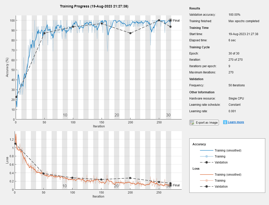
Train the network using the architecture defined bylayers, the training data, and the training options. By default,trainNetworkuses a GPU if one is available, otherwise, it uses a CPU. Training on a GPU requires Parallel Computing Toolbox™ and a supported GPU device. For information on supported devices, seeGPU Computing Requirements(Parallel Computing Toolbox). You can also specify the execution environment by using the'ExecutionEnvironment'name-value pair argument oftrainingOptions.

The training progress plot shows the mini-batch loss and accuracy and the validation loss and accuracy. For more information on the training progress plot, seeMonitor Deep Learning Training Progress.

net = trainNetwork(tblTrain,labelName,layers,options);

Figure Training Progress (03-Mar-2023 09:07:26) contains 2 axes objects and another object of type uigridlayout. Axes object 1 with xlabel Iteration, ylabel Loss contains 10 objects of type patch, text, line. Axes object 2 with xlabel Iteration, ylabel Accuracy (%) contains 10 objects of type patch, text, line.

Test Network

Predict the labels of the test data using the trained network and calculate the accuracy. Specify the same mini-batch size used for training.

YPred = classify(net,tblTest(:,1:end-1),'MiniBatchSize',miniBatchSize);

Calculate the classification accuracy. The accuracy is the proportion of the labels that the network predicts correctly.

YTest = tblTest{:,labelName}; accuracy = sum(YPred == YTest)/numel(YTest)

accuracy = 0.9688

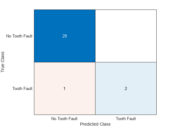
View the results in a confusion matrix.

figure confusionchart(YTest,YPred)

Figure contains an object of type ConfusionMatrixChart.