Space debris scenario

There are more than 30,000 large debris objects (with diameter larger than 10cm) and more than 1 million smaller debris objects in Low Earth Orbit (LEO) [1]. This debris can be dangerous for human activities in space, damage operational satellites, and force time sensitive and costly avoidance maneuvers. As space activity increases, reducing and monitoring the space debris becomes crucial.

You can use Sensor Fusion and Tracking Toolbox™ to model the debris trajectories, generate synthetic radar detections of this debris, and obtain position and velocity estimates of each object.

First, create a tracking scenario and set the random seed for repeatable results.

s = rng; rng(2020); scene = trackingScenario('IsEarthCentered',true,'InitialAdvance','UpdateInterval',...'StopTime', 3600,'UpdateRate', 0.1);

You use the Earth-Centered-Earth-Fixed (ECEF) reference frame. The origin of this frame is at the center of the Earth and the Z axis points toward the north pole. The X axis points towards the intersection of the equator and the Greenwich meridian. The Y axis completes the right-handed system. Platform positions and velocities are defined using Cartesian coordinates in this frame.

Define debris motion model

ThehelperMotionTrajectoryclass used in this example defines debris object trajectories using a custom motion model function.

Trajectories of space objects rotating around the Earth can be approximated with a Keplerian model, which assumes that Earth is a point-mass body and the objects orbiting around the earth have negligible masses. Higher order effects in Earth gravitational field and environmental disturbances are not accounted for. Since the equation of motion is expressed in ECEF frame which is a non-inertial reference frame, the Coriolis and centripetal forces are accounted for.

The ECEF debris object acceleration vector is

$$\stackrel{\to }{\mathit{a}}=\frac{-\mu }{{\mathit{r}}^3}\stackrel{\to }{\mathit{r}}-2\stackrel{\to }{\Omega }\times \frac{\mathrm{d}}{\mathrm{d}\mathit{t}}\stackrel{\to }{\mathit{r}}-\stackrel{\to }{\Omega }\times \left(\stackrel{\to }{\Omega }\times \stackrel{\to }{\mathit{r}}\right)$$,

where $\mu$is the standard gravitational parameter of the Earth, $\stackrel{\to }{\mathit{r}}$is the ECEF debris object position vector, $\mathit{r}$is the norm of the position vector, and $\stackrel{\to }{\Omega }$is the Earth rotation vector.

The functionkeplerorbitprovided below uses a 4th order Runge-Kutta numerical integration of this equation to propagate the position and velocity in time.

First, we create initial positions and velocities for the space debris objects. This is done by obtaining the traditional orbital elements (semi-major axis, eccentricity, inclination, longitude of the ascending node, argument of periapsis, and true anomaly angles) of these objects from random distributions. Then convert these orbital elements to position and velocity vectors by using the supporting functionoe2rv.

% Generate a population of debrisnumDebris = 100; range = 7e6 + 1e5*randn(numDebris,1); ecc = 0.015 + 0.005*randn(numDebris,1); inc = 80 + 10*rand(numDebris,1); lan = 360*rand(numDebris,1); w = 360*rand(numDebris,1); nu = 360*rand(numDebris,1);% Convert to initial position and velocityfori = 1:numDebris [r,v] = oe2rv(range(i),ecc(i),inc(i),lan(i),w(i),nu(i)); data(i).InitialPosition = r;%#okdata(i).InitialVelocity = v;%#okend% Create platforms and assign them trajectories using the keplerorbit motion modelfori=1:numDebris debris(i) = platform(scene);%#okdebris(i).Trajectory = helperMotionTrajectory(@keplerorbit,...'SampleRate',0.1,...% integration step 10sec'Position',data(i).InitialPosition,...'Velocity',data(i).InitialVelocity);%#okend

Model space surveillance radars

In this example, we define four antipodal stations with fan-shaped radar beams looking into space. The fans cut through the orbits of debris objects to maximize the number of object detections. A pair of stations are located in the Pacific ocean and in the Atlantic ocean, whereas a second pair of surveillance stations are located near the poles. Having four dispersed radars allows for the re-detection of space debris to correct their position estimates and also acquiring new debris detections.

% Create a space surveillance station in the Pacific oceanstation1 = platform(scene,'Position',[10 180 0]);% Create a second surveillance station in the Atlantic oceanstation2 = platform(scene,'Position',[0 -20 0]);% Near the North Pole, create a third surveillance station in Icelandstation3 = platform(scene,'Position',[65 -20 0]);% Create a fourth surveillance station near the south polestation4 = platform(scene,'Position',[-90 0 0]);

Each station is equipped with a radar modeled with afusionRadarSensorobject. In order to detect debris objects in the LEO range, the radar has the following requirements:

% Create fan-shaped monostatic radars to monitor space debris objectsradar1 = fusionRadarSensor(1,...'UpdateRate',0.1,...10 sec'ScanMode','No scanning',...'MountingAngles',[0 90 0],...look up'FieldOfView',[120;30],...degrees'ReferenceRange',2e6,...m'RangeLimits', [0 2e6],...'ReferenceRCS', 10,...dBsm'HasFalseAlarms',false,...'HasElevation',true,...'AzimuthResolution',0.01,...degrees'ElevationResolution',0.01,...degrees'RangeResolution',100,...m'HasINS',true,...'DetectionCoordinates','Scenario'); station1.Sensors = radar1; radar2 = clone(radar1); radar2.SensorIndex = 2; station2.Sensors = radar2; radar3 = clone(radar1); radar3.SensorIndex = 3; station3.Sensors = radar3; radar4 = clone(radar1); radar4.SensorIndex = 4; station4.Sensors = radar4;

Visualize the ground truth with trackingGlobeViewer

You usetrackingGlobeViewerto visualize all the elements defined in the tracking scenario: individual debris objects and their trajectories, radar fans, radar detections, and tracks.

f = uifigure; viewer = trackingGlobeViewer(f,'Basemap','satellite','ShowDroppedTracks',false);% Add info box on top of the globe viewerinfotext = simulationInfoText(0,0,0); infobox = uilabel(f,'Text',infotext,'FontColor',[1 1 1],“字形大小”,11,...'Position',[10 20 300 70],'Visible','on');% Show radar beams on the globecovcon = coverageConfig(scene); plotCoverage(viewer,covcon,'ECEF');whileadvance(scene) infobox.Text = simulationInfoText(scene.SimulationTime, 0, numDebris); plotPlatform(viewer, debris,'ECEF');end%Take a snapshot of the scenariosnapshot(viewer);

On the virtual globe, you can see the space debris represented by white dots with individual trailing trajectories shown by white lines. Most of the generated debris objects are on orbits with high inclination angles close to 80 deg.

The trajectories are plotted in ECEF coordinates, and therefore the entire trajectory rotates towards the west due to Earth rotation. After several orbit periods, all space debris pass through the surveillance beams of the radars.

Simulate synthetic detections and track space debris

The sensor models use the ground truth to generate synthetic detections. Call thedetectmethod on the tracking scenario to obtain all the detections in the scene.

A multi-object trackertrackerJPDAis used to create new tracks, associate detections to existing tracks, estimate their state, and delete divergent tracks. Setting the propertyHasDetectableTrackIDsInputto true allows the tracker to accept an input that indicates whether a tracked object is detectable in the surveillance region. This is important for not penalizing tracks that are propagated outside of the radar surveillance areas. The utility functionisDetectablecalculates which tracks are detectable at each simulation step.

Additionally, a utility functiondeleteBadTracksis used to delete divergent tracks faster.

% Define Trackertracker = trackerJPDA('FilterInitializationFcn',@initKeplerUKF,...'HasDetectableTrackIDsInput',true,...'ClutterDensity',1e-20,...'AssignmentThreshold',1e3,...'DeletionThreshold',[7 10]);% Reset scenario, seed, and globe displayrestart(scene); scene.StopTime = 1800;% 30 minclear(viewer);% Reduce history depth for debris查看器。PlatformHistoryDepth = 2;% Show 10-sigma covariance ellipses for better visibility查看器。NumCovarianceSigma = 10; plotCoverage(viewer,covcon,'ECEF');% Initialize tracksconfTracks = objectTrack.empty(0,1);whileadvance(scene) plotPlatform(viewer, debris); time = scene.SimulationTime;% Generate detectionsdetections = detect(scene); plotDetection(viewer, detections,'ECEF');% Generate and update tracksdetectableInput = isDetectable(tracker,time, covcon);ifisLocked(tracker) || ~isempty(detections) [confTracks, ~, allTracks,info] = tracker(detections,time,detectableInput); confTracks = deleteBadTracks(tracker,confTracks); plotTrack(viewer, confTracks,'ECEF');endinfobox.Text = simulationInfoText(time, numel(confTracks), numDebris);% Move camera during simulation and take snapshotsswitch时间case100 campos(viewer,[90 150 5e6]); camorient(viewer,[0 -65 345]); drawnow im1 = snapshot(viewer);case270 campos(viewer,[60 -120 2.6e6]); camorient(viewer, [20 -45 20]); drawnowcase380 campos(viewer,[60 -120 2.6e6]); camorient(viewer, [20 -45 20]); drawnow im2 = snapshot(viewer);case400% resetcampos(viewer,[17.3 -67.2 2.400e7]); camorient(viewer, [360 -90 0]); drawnowcase1500 campos(viewer,[54 2.3 6.09e6]); camorient(viewer, [0 -73 348]); drawnowcase1560 im3 = snapshot(viewer); drawnowendend%恢复随机种子rng(s);

imshow(im1);

On the first snapshot, you can see an object being tracked as track T1 in yellow. This object was only detected twice, which was not enough to reduce the uncertainty of the track. Therefore, the size of its covariance ellipse is relatively large. You can also observe another track T2 in blue, which is detected by the sensor several times. As a result, its corresponding covariance ellipse is much smaller since more detections were used to correct the state estimate.

imshow(im2);

A few minutes later, as seen on the snapshot above, T1 was deleted because the uncertainty of the track has grown too large without detections. On the other hand, the second track T2 survived due to the additional detections.

imshow(im3)

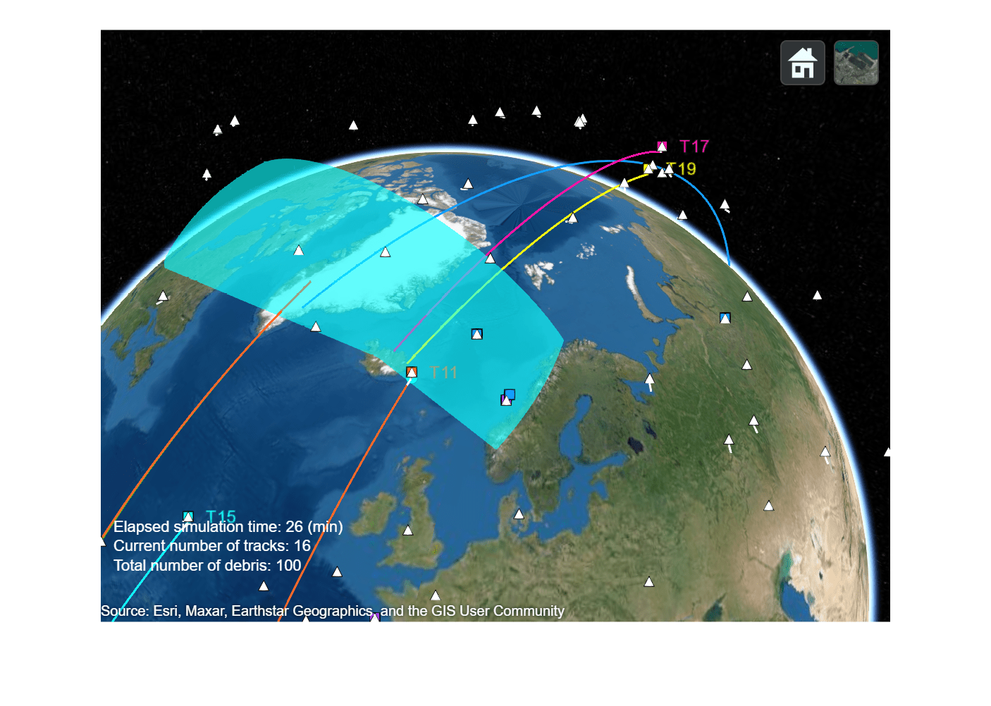
In the screenshot above, you can see that track T15 (in light blue) is about to enter the radar surveillance area. Track T11 (in orange) was just updated with a detection, which reduced the uncertainty of its estimated position and velocity. With radar station configuration, after 30 minutes of surveillance, 18 tracks were initialized and confirmed out of the 100 debris objects. If you increase the simulation time, the radars will cover 360 degrees in space and eventually more debris can be tracked. Different radar station locations and configurations could be explored to increase the number of tracked objects.

Summary

In this example you have learned how to specify your own motion model to move platforms in a tracking scenario and how to use them to setup a tracker. This enables you to apply sensor fusion and tracking techniques offered in this toolbox to a wider range of applications, such as the problem of modelling and tracking space debris in an Earth-Centered-Earth-Fixed coordinate frame as shown in this example.

Supporting functions

The motion model used in this example is presented below. The state is the ECEF positions and velocities of the object[x; vx; y; vy; z; vz].

functionstate = keplerorbit(state,dt)% keplerorbit performs numerical integration to predict the state of% keplerian bodies. The state is [x;vx;y;vy;z;vz]% Runge-Kutta 4 integration method:k1 =开普勒(状态);k2 =凯普ler(state + dt*k1/2); k3 = kepler(state + dt*k2/2); k4 = kepler(state + dt*k3); state = state + dt*(k1+2*k2+2*k3+k4)/6;functiondstate=kepler(state) x =state(1,:); vx = state(2,:); y=state(3,:); vy = state(4,:); z=state(5,:); vz = state(6,:); mu = 398600.4405*1e9;% m^3 s^-2omega = 7.292115e-5;% rad/sr = norm([x y z]); g = mu/r^2;% Coordinates are in a non-intertial frame, account for Coriolis% and centripetal accelerationax = -g*x/r + 2*omega*vy + omega^2*x; ay = -g*y/r - 2*omega*vx + omega^2*y; az = -g*z/r; dstate = [vx;ax;vy;ay;vz;az];endend

initKeplerUKFinitializes a tracking filter with your own motion model. In this example, we use the same motion model that establishes ground truth,keplerorbit.

functionfilter = initKeplerUKF(detection)% assumes radar returns [x y z]measmodel= @(x,varargin) x([1 3 5],:); detNoise = detection.MeasurementNoise; sigpos = 0.4;% msigvel = 0.4;% m/s^2meas = detection.Measurement; initState = [meas(1); 0; meas(2); 0; meas(3);0]; filter = trackingUKF(@keplerorbit,measmodel,initState,...'StateCovariance', diag(repmat([10, 10000].^2,1,3)),...'ProcessNoise',diag(repmat([sigpos, sigvel].^2,1,3)),...'MeasurementNoise',detNoise);end

oe2rvconverts a set of 6 traditional orbital elements to position and velocity vectors.

function[r,v] = oe2rv(a,e,i,lan,w,nu)% Reference: Bate, Mueller & White, Fundamentals of Astrodynamics Sec 2.5mu = 398600.4405*1e9;% m^3 s^-2% Express r and v in perifocal systemcnu = cosd(nu); snu = sind(nu); p = a*(1 - e^2); r = p/(1 + e*cnu); r_peri = [r*cnu ; r*snu ; 0]; v_peri = sqrt(mu/p)*[-snu ; e + cnu ; 0];% Tranform into Geocentric Equatorial frame家族= cosd(局域网);超人=信德(局域网);连续波= cosd (w);sw = sind(w); ci = cosd(i); si = sind(i); R = [ clan*cw-slan*sw*ci , -clan*sw-slan*cw*ci , slan*si;...slan*cw+clan*sw*ci , -slan*sw+clan*cw*ci , -clan*si;...sw*si , cw*si , ci]; r = R*r_peri; v = R*v_peri;end

isDetectableis used in the example to determine which tracks are detectable at a given time.

functiondetectInput = isDetectable(tracker,time,covcon)if～isLocked(tracker) detectInput = zeros(0,1,'uint32');returnendtracks = tracker.predictTracksToTime('all',time);ifisempty(tracks) detectInput = zeros(0,1,'uint32');elsealltrackid = [tracks.TrackID]; isDetectable = zeros(numel(tracks),numel(covcon),'logical');fori = 1:numel(tracks) track = tracks(i); pos_scene = track.State([1 3 5]);forj=1:numel(covcon) config = covcon(j);% rotate position to sensor frame:d_scene = pos_scene(:) - config.Position(:); scene2sens = rotmat(config.Orientation,'frame'); d_sens = scene2sens*d_scene(:); [az,el] = cart2sph(d_sens(1),d_sens(2),d_sens(3));ifabs(rad2deg(az)) <= config.FieldOfView(1)/2 && abs(rad2deg(el)) < config.FieldOfView(2)/2 isDetectable(i,j) = true;elseisDetectable(i,j) = false;endendenddetectInput = alltrackid(any(isDetectable,2))';endend

deleteBadTracksis used to remove tracks that obviously diverged. Specifically, diverged tracks in this example are tracks whose current position has fallen on the surface of the earth and tracks whose covariance has become too large.

functiontracks = deleteBadTracks(tracker,tracks)% remove divergent tracks:% - tracks with covariance > 4*1e8 (20 km standard deviation)% - tracks with estimated position outside of LEO boundsn = numel(tracks); toDelete = zeros(1,n,'logical');fori=1:numel(tracks) [pos, cov] = getTrackPositions(tracks(i),[ 1 0 0 0 0 0 ; 0 0 1 0 0 0; 0 0 0 0 1 0]);ifnorm(pos) < 6500*1e3 || norm(pos) > 8500*1e3 || max(cov,[],'all') > 4*1e8 deleteTrack(tracker,tracks(i).TrackID); toDelete(i) =true;endendtracks(toDelete) = [];end

simulationInfoTextis used to display the simulation time, the number of debris, and the current number of tracks in the scenario.

function文本= simulationInfoText(时间、numTracks numDebris) text = vertcat(string(['Elapsed simulation time: 'num2str(round(time/60))' (min)']),...string(['Current number of tracks: 'num2str(numTracks)]),...string(['Total number of debris: 'num2str(numDebris)])); drawnowlimitrateend

References

[1]https://www.esa.int/Safety_Security/Space_Debris/Space_debris_by_the_numbers