refit
Class:FeatureSelectionNCARegression
Refit neighborhood component analysis (NCA) model for regression
Syntax
mdlrefit =refit(mdl,Name,Value)
Description
mdlrefit= refit(mdl,Name,Value)mdl, with modified parameters specified by one or moreName,Valuepair arguments.
Input Arguments
mdl—Neighborhood component analysis model for regression
FeatureSelectionNCARegressionobject
Neighborhood component analysis model or classification, specified as aFeatureSelectionNCARegressionobject.
Name-Value Arguments
Specify optional pairs of arguments asName1=Value1,...,NameN=ValueN, whereNameis the argument name andValueis the corresponding value. Name-value arguments must appear after other arguments, but the order of the pairs does not matter.
Before R2021a, use commas to separate each name and value, and encloseNamein quotes.
FitMethod—Method for fitting the model
mdl。FitMethod(default) |'exact'|'none'|'average'
Method for fitting the model, specified as the comma-separated pair consisting of'FitMethod'and one of the following.
'exact'— Performs fitting using all of the data.'none'— No fitting. Use this option to evaluate the generalization error of the NCA model using the initial feature weights supplied in the call tofsrnca.'average'— The function divides the data into partitions (subsets), fits each partition using theexactmethod, and returns the average of the feature weights. You can specify the number of partitions using theNumPartitionsname-value pair argument.
Example:'FitMethod','none'
Lambda—Regularization parameter
mdl。Lambda(default) |non-negative scalar value
Regularization parameter, specified as the comma-separated pair consisting of'Lambda'and a non-negative scalar value.
Fornobservations, the bestLambdavalue that minimizes the generalization error of the NCA model is expected to be a multiple of 1/n
Example:'Lambda',0.01
Data Types:double|single
Solver—Solver type
mdl。Solver(default) |'lbfgs'|'sgd'|'minibatch-lbfgs'
Solver type for estimating feature weights, specified as the comma-separated pair consisting of'Solver'and one of the following.
'lbfgs'— Limited memory BFGS (Broyden-Fletcher-Goldfarb-Shanno) algorithm (LBFGS algorithm)'sgd'— Stochastic gradient descent'minibatch-lbfgs'——与LBFGS随机梯度下降算法applied to mini-batches
Example:'solver','minibatch-lbfgs'
InitialFeatureWeights—Initial feature weights
mdl。InitialFeatureWeights(default) |p-by-1 vector of real positive scalar values
Initial feature weights, specified as the comma-separated pair consisting of'InitialFeatureWeights'and ap-by-1 vector of real positive scalar values.
Data Types:double|single
Verbose—Indicator for verbosity level
mdl。Verbose(default) |0|1|>1
Indicator for verbosity level for the convergence summary display, specified as the comma-separated pair consisting of'Verbose'and one of the following.
0 — No convergence summary
1 — Convergence summary including iteration number, norm of the gradient, and objective function value.
>1 — More convergence information depending on the fitting algorithm
When using solver
'minibatch-lbfgs'and verbosity level >1, the convergence information includes iteration log from intermediate mini-batch LBFGS fits.
Example:'Verbose',2
Data Types:double|single
GradientTolerance—Relative convergence tolerance
mdl。GradientTolerance(default) |positive real scalar value
Relative convergence tolerance on the gradient norm for solverlbfgs, specified as the comma-separated pair consisting of'GradientTolerance'and a positive real scalar value.
Example:'GradientTolerance',0.00001
Data Types:double|single
InitialLearningRate—Initial learning rate for solversgd
mdl。InitialLearningRate(default) |positive real scalar value
Initial learning rate for solversgd, specified as the comma-separated pair consisting of'InitialLearningRate'and a positive scalar value.
When using solver type'sgd', the learning rate decays over iterations starting with the value specified for'InitialLearningRate'.
Example:'InitialLearningRate',0.8
Data Types:double|single
PassLimit—Maximum number of passes for solver'sgd'
mdl。PassLimit(default) |positive integer value
Maximum number of passes for solver'sgd'(stochastic gradient descent), specified as the comma-separated pair consisting of'PassLimit'and a positive integer. Every pass processessize(mdl.X,1)observations.
Example:'PassLimit',10
Data Types:double|single
IterationLimit—Maximum number of iterations
mdl。IterationLimit(default) |positive integer value
Maximum number of iterations, specified as the comma-separated pair consisting of'IterationLimit'and a positive integer.
Example:'IterationLimit',250
Data Types:double|single
Output Arguments
mdlrefit— Neighborhood component analysis model for regression
FeatureSelectionNCARegressionobject
Neighborhood component analysis model or classification, returned as aFeatureSelectionNCARegressionobject. You can either save the results as a new model or update the existing model asmdl = refit(mdl,Name,Value).
Examples
Refit NCA Model for Regression with Modified Settings
Load the sample data.
load('robotarm.mat')
Therobotarm(pumadyn32nm) dataset is created using a robot arm simulator with 7168 training and 1024 test observations with 32 features [1], [2]. This is a preprocessed version of the original data set. Data are preprocessed by subtracting off a linear regression fit followed by normalization of all features to unit variance.
Compute the generalization error without feature selection.
nca = fsrnca(Xtrain,ytrain,'FitMethod','none','Standardize',1); L = loss(nca,Xtest,ytest)
L = 0.9017
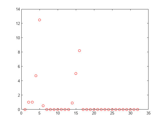
Now, refit the model and compute the prediction loss with feature selection, with
= 0 (no regularization term) and compare to the previous loss value, to determine feature selection seems necessary for this problem. For the settings that you do not change,refituses the settings of the initial modelnca. For example, it uses the feature weights found inncaas the initial feature weights.
nca2 = refit(nca,'FitMethod','exact','Lambda',0); L2 = loss(nca2,Xtest,ytest)
L2 = 0.1088
The decrease in the loss suggests that feature selection is necessary.
Plot the feature weights.
figure() plot(nca2.FeatureWeights,'ro')

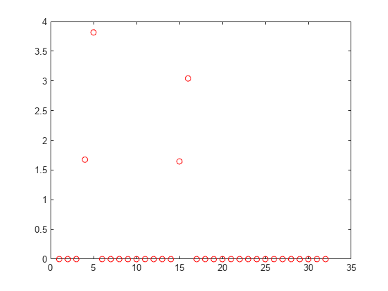
Tuning the regularization parameter usually improves the results. Suppose that, after tuning
using cross-validation as inTune Regularization Parameter in NCA for Regression, the best
value found is 0.0035. Refit thencamodel using this
value and stochastic gradient descent as the solver. Compute the prediction loss.
nca3 = refit(nca2,'FitMethod','exact','Lambda',0.0035,...'Solver','sgd'); L3 = loss(nca3,Xtest,ytest)
L3 = 0.0573
Plot the feature weights.
figure() plot(nca3.FeatureWeights,'ro')

After tuning the regularization parameter, the loss decreased even more and the software identified four of the features as relevant.
References
[1] Rasmussen, C. E., R. M. Neal, G. E. Hinton, D. van Camp, M. Revow, Z. Ghahramani, R. Kustra, and R. Tibshirani. The DELVE Manual, 1996,https://mlg.eng.cam.ac.uk/pub/pdf/RasNeaHinetal96.pdf
Version History
Introduced in R2016b
See Also
Ouvrir l'exemple
Vous possédez une version modifiée de cet exemple. Souhaitez-vous ouvrir cet exemple avec vos modifications ?
Commande MATLAB
Vous avez cliqué sur un lien qui correspond à cette commande MATLAB :
Pour exécuter la commande, saisissez-la dans la fenêtre de commande de MATLAB. Les navigateurs web ne supportent pas les commandes MATLAB.

Select a Web Site
Choose a web site to get translated content where available and see local events and offers. Based on your location, we recommend that you select:.
You can also select a web site from the following list:
How to Get Best Site Performance
Select the China site (in Chinese or English) for best site performance. Other MathWorks country sites are not optimized for visits from your location.
Americas
- América Latina(Español)
- Canada(English)
- United States(English)
Europe
- Belgium(English)
- Denmark(English)
- Deutschland(Deutsch)
- España(Español)
- Finland(English)
- France(Français)
- Ireland(English)
- Italia(Italiano)
- Luxembourg(English)
- Netherlands(English)
- Norway(English)
- Österreich(Deutsch)
- Portugal(English)
- Sweden(English)
- Switzerland
- United Kingdom(English)