Create Thin Dipole

The default dipole has a width of 10 cm. Reduce the width to 1 cm and make the change to the dipole parameter Width.

mydipole = dipole; w = 1e-2; mydipole.Width = w;

Calculate Baseline Impedance

Calculate and store the impedance and the number of triangular facets in the mesh when using the default mesh. Since the dipole length is 2 m, we choose the analysis frequency as half-wavelength frequency $$f=c/(2*l)$$, where c, is the speed of light.

c = 2.99792458e8; f = c/(2*mydipole.Length); Zbaseline = impedance(mydipole,f); meshdata = mesh(mydipole); Nbaseline = meshdata.NumTriangles; Mbaseline = meshdata.MaxEdgeLength;

Define Analysis Parameters

Create parameters to store impedance, the relative change in impedance and the mesh size.

Zin = Zbaseline; numTri = Nbaseline; Ztemp = Zin(1);

Impact of Mesh Accuracy on Antenna Impedance

The triangular surface mesh implies a discretization of the surface geometry into small planar triangles. All antenna surfaces in the Antenna Toolbox� are discretized into triangles. You can evaluate the accuracy of the simulation results by uniformly refining the mesh. To specify the resolution of the mesh, provide the size of the maximum edge length, i.e. the longest side of a triangle among all triangles in the mesh, prior to analysis.

For each value of the maximum edge length, update the mesh, calculate the impedance at the predefined operating frequency, and calculate the number of triangles in the mesh. Store the impedance and the number of triangles in the mesh for subsequent analysis. Finally, calculate the relative change in the antenna impedance between subsequent mesh refinements until a desired convergence criterion is met.

exptol = .002; tolCheck = []; n = 1; nmax = 12; pretol = 1; ShrinkFactor = 0.96;while(n < nmax+1)&&(pretol > exptol) Mbaseline(n+1)=Mbaseline(n)*ShrinkFactor^(n-1); meshdata = mesh(mydipole,'MaxEdgeLength',Mbaseline(n+1)); numTri(n+1) = meshdata.NumTriangles;% Check if mesh has changed and only then calculate impedanceifnumTri(n+1)~=numTri(n) Zin(n+1) = impedance(mydipole,f); Zchange = abs((Zin(n+1)-Ztemp)/Zin(n+1));elseZin(n+1) = Zin(n); Zchange = pretol;endtolCheck(n) = Zchange;%#okpretol = tolCheck(n); Ztemp = Zin(n+1); n = n+1;endtolValue = exptol.*ones(1,n); tolCheck = [nan tolCheck];

Impedance of Dipole with Finer Meshes

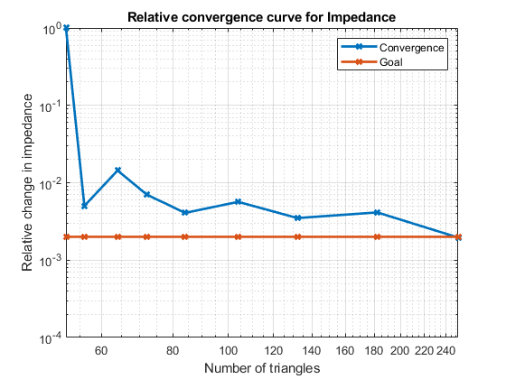
最后的分析, the resistance, $$R_{in}$$ $\approx 84\Omega$and reactance, $$X_{in}$$ $\approx 45\Omega$. This value is in good agreement with the results reported in [1], [3]. Better results are obtained with an adaptive mesh refinement algorithm, which implies selective mesh refinement in the domain of a maximum numerical error. For this case, the relative convergence curve is shown below

figure; loglog(numTri,tolCheck,“- x”,'LineWidth',2) holdonloglog(numTri,tolValue,“- x”,'LineWidth',2) axis([min(numTri),max(numTri),10^-4,1]) gridonxlabel('Number of triangles') ylabel('Relative change in impedance') legend('Convergence','Goal') title('Relative convergence curve for Impedance')

See Also

Analysis of Monopole Impedance

References

[1] S. N. Makarov, 'Antenna and EM Modeling with MATLAB,' p.66, Wiley, 2002.

[2] C. A. Balanis, 'Antenna Theory. Analysis and Design,' p.514, Wiley, New York, 3rd Edition, 2005

[3] R. C. Hansen, "Carter Dipoles and Resonant Dipoles," Proceedings of the Antenna Application Symposium, Allerton Park, Monticello, IL, pp.282-284, Sep. 21-23rd 2010.