Approximate Model with Unstable or Near-Unstable Pole

This example shows how to compute a reduced-order approximation of a system when the system has unstable or near-unstable poles.

When computing a reduced-order approximation, thebalredcommand (or theModel Reducer波兰人因为doi app)并不能消除不稳定ng so would fundamentally change the system dynamics. Instead, the software decomposes the model into stable and unstable parts and reduces the stable part of the model.

If your model has near-unstable poles, you might want to ensure that the reduced-order approximation preserves these dynamics. This example shows how to use theOffsetoption ofbalredto preserve poles that are close to the stable-unstable boundary. You can achieve the same result in theModel Reducerapp, on theBalanced Truncationtab, underOptions, using theOffsetfield, as shown:

Load a model with unstable and near-unstable poles.

load('reduce.mat','gasf35unst')

gasf35unstis a 25-state SISO model with two unstable poles (Re(s) > 0). Examine the system poles to find the near-unstable poles.

pzplot (gasf35unst) axis([-0.0015 0.0015 -0.0005 0.0005])

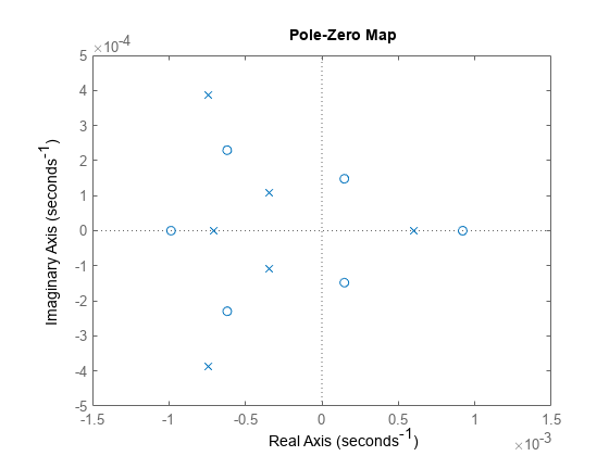
The pole-zero plot shows several poles (marked byx) that fall in the left half-plane, but relatively close to the imaginary axis. These are the near-unstable poles. Two of these fall within 0.0005 of instability. Three more fall within 0.001 of instability.

Examine a Hankel singular-value plot of the model.

hsvplot(gasf35unst)

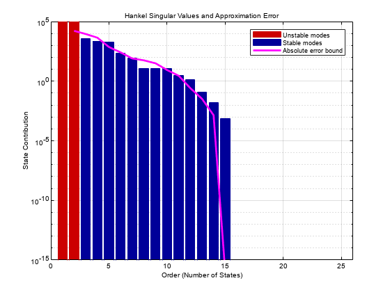
The plot shows the two unstable modes, but you cannot easily determine the energy contribution of the near-unstable poles. In your application, you might want to reduce the model without discarding those poles nearest to instability, even if they are of relatively low energy. Use theOffsetoption ofbalredto calculate a reduced-order system that preserves the two stable poles that are closest to the imaginary axis. TheOffsetoption sets the boundary between poles thatbalredcan discard, and poles thatbalredmust preserve (treat as unstable).

opts = balredOptions('Offset',0.0005); gasf_arr = balred(gasf35unst,[10 15],opts);

Providingbalredan array of target approximation orders[10 15]causesbalredto return an array of approximated models. The arraygasf_arrcontains two models, a 10th-order and a 15th-order approximation ofgasf35unst. In both approximations,balreddoes not discard the two unstable poles or the two nearly-unstable poles.

Compare the reduced-order approximations to the original model.

bodeplot(gasf35unst,gasf_arr,'r--')

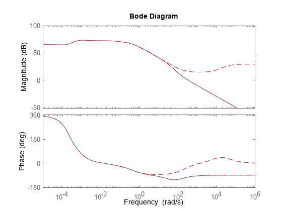
The 15th order approximation is a good frequency-domain match to the original model. However, the 10th-order approximation shows changes in high-frequency dynamics, which might be too large to be acceptable. The 15th-order approximation is likely a better choice.

See Also

Functions

• balred|hsvplot

Live Editor Tasks

• Reduce Model Order

Related Topics

• Balanced Truncation Model Reduction
• Approximate Model by Balanced Truncation at the Command Line
• Frequency-Limited Balanced Truncation