Measurement of Pulse and Transition Characteristics

打开实时脚本

此示例显示了如何分析脉冲和过渡和计算指标，包括上升时间，秋季时间，振荡速率，过冲，散发，脉冲宽度，占空比，占空比和脉冲周期。

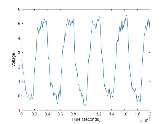
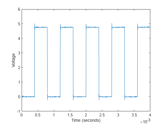
噪音的时钟信号

First view the samples from a noisy clock signal.

loadclocksigclock1时间1Fsplot(time1,clock1) xlabel(“时间（秒）”）ylabel（'Voltage')

Figure contains an axes object. The axes object contains an object of type line.

估计国家一级

利用Statelevelswith no output argument to visualize the state levels. The histogram method is used to estimate the state levels with these steps:

确定数据的最小和最大幅度。
对于指定数量的直方图箱，请确定箱宽度，这是振幅范围与箱数的比率。使用可选的输入参数来指定直方图箱和直方图边界的数量。
将数据值分类到直方图箱中。
确定具有非零计数的最低和最高索引直方图箱。
Divide the histogram into two subhistograms.
通过确定上下直方图的模式或均值来计算状态水平。

Statelevels(clock1)

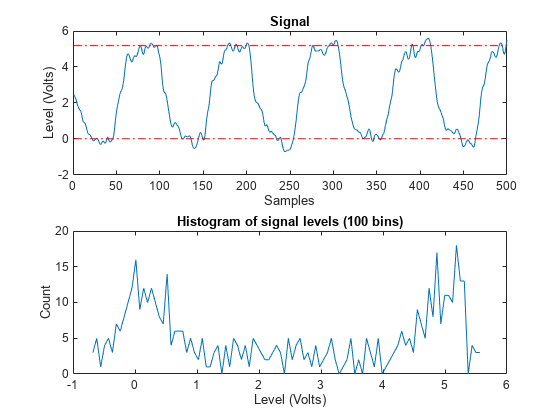
图状态级信息包含2个轴对象。轴对象1具有信号级别（100箱）的标题直方图包含类型线的对象。带有标题信号的轴对象2包含3个类型行的对象。

ans =1×20.0138 5.1848

计算的直方图分为第一个和最后一个箱之间的两个相等大小的区域。直方图每个区域的模式作为命令窗口中的估计状态级值返回。

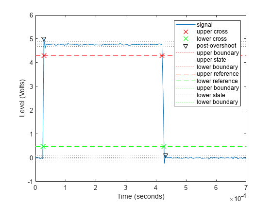
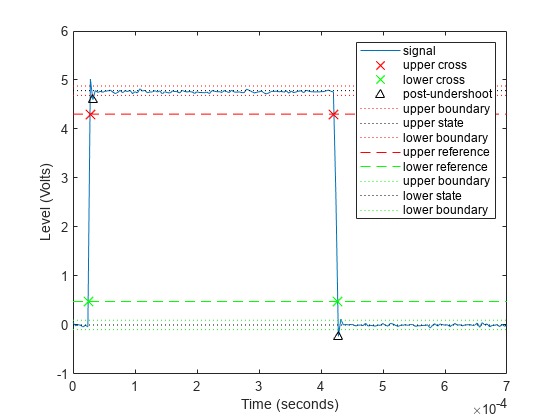
Measure Rise Time, Fall Time and Slew Rate

Risetimeis the duration between the instants where the rising transition of each pulse crosses from the lower to the upper reference levels.落下timeis the duration between the instants where the falling transition of each pulse crosses from the upper to the lower reference levels. The default reference levels for computing rise time and fall time are set at 10% and 90% of the waveform amplitude.

利用上升时间with no output argument to visualize the rise time of positive-going edges. Then, use秋季没有输出参数可视化负边缘的秋季时间。将参考级别指定为[2080]和状态级别[05]。

上升时间(clock1,time1)

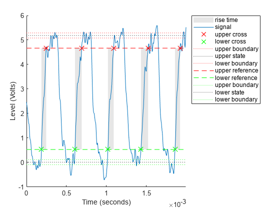
图上升时间图包含一个轴对象。轴对象包含12个类型补丁的对象。这些对象代表上升时间，信号，上十字，下部十字，上边界，上部状态，下边界，下边界，上引用，下引用，下部状态。

ans =5×110^-4× 0.5919 0.8344 0.7185 0.8970 0.6366

秋季(clock1,time1,“PercentReferenceLevels'，[20 80]，'StateLevels'，[0 5]）

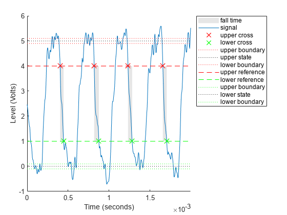
图秋季时间图包含一个轴对象。轴对象包含12个类型补丁的对象。这些物体代表秋季时间，信号，上十字，下部十字，上边界，上部状态，下边界，下边界，上引用，下引用，下部状态。

ans =4×110^-4×0.4294 0.5727 0.5032 0.4762

Obtain measurements programmatically by calling functions with one or more output arguments. For uniformly sampled data, you can provide a sample rate in place of the time vector. Useslewrate测量每个正进行或负面边缘的斜率。

sr = slewrate（clock1（1：100），fs）

SR = 7.0840E+04

分析过冲和下调

Now view data from a clock with significant overshoot and undershoot.

loadclocksigclock2时间2Fsplot(time2,clock2) xlabel(“时间（秒）”）ylabel（'Voltage')

图秋季时间图包含一个轴对象。The axes object contains an object of type line.

Underdamped clock signals have overshoots. Overshoots are expressed as a percentage of the difference between state levels. Overshoots can occur just after an edge, at the start of the post-transition aberration region. Use theovershoot功能以测量这些后弹后的超声。

overshoot(clock2(95:270),Fs)

ans =2×14.9451 2.5399

legend('地点','东北')

图超声图包含一个轴对象。轴对象包含12个类型行的对象。这些对象代表信号，上十字，下部十字，后冲后，上边界，上部状态，下边界，上部参考，下引用，下部状态。

Overshoots may also occur just before an edge, at the end of the pre-transition aberration region. These are called preshoot overshoots.

Similarly, you can measure undershoots in the pre- and post-aberration regions. Undershoots are also expressed as a percentage of the difference between the state levels. Use optional input arguments to specify the regions in which to measure aberrations.

surdshoot（clock2（95：270），fs，'Region','Postshoot')

ans =2×13.8499 4.9451

legend('地点','东北')

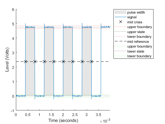
Figure Undershoot Plot contains an axes object. The axes object contains 12 objects of type line. These objects represent signal, upper cross, lower cross, post-undershoot, upper boundary, upper state, lower boundary, upper reference, lower reference, lower state.

Measure Pulse Width and Duty Cycle

宽度是每个脉冲的第一和第二过渡的中期交叉点之间的持续时间。利用pulsewidth没有输出参数来绘制突出显示的脉冲宽度。指定正极性。

pulsewidth(clock2, time2,'Polarity','Positive');

图脉冲宽度图包含一个轴对象。轴对象包含10个类型补丁的对象。这些对象代表脉冲宽度，信号，中十字，上边界，上部状态，下边界，中间参考，下部状态。

利用dutycycle计算每个负极性脉冲的脉冲宽度与脉冲周期的比率。

d = tuncycle（clock2，time2，'Polarity','消极的')

d =3×10.4979 0.5000 0.5000

利用pulseperiodto obtain the periods of each cycle of the waveform. Theperiod是电流脉冲的第一个过渡与下一个脉冲的第一个跃迁之间的持续时间。使用此信息来计算其他指标，例如波形的平均频率或总观察到的抖动。

pp = pulseperiod(clock2, time2); avgFreq = 1./mean(pp)

AVGFREQ = 1.2500E+03

totalJitter = std(pp)

totalJitter = 1.9866e-06