Introduction

Adaptive system identification is one of the main applications of adaptive filtering. This example showcases system identification using an RLS filter. The example's workflow is depicted below:

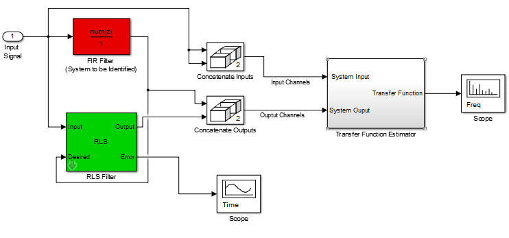
未知的系统是由一个低通滤波器建模冷杉费尔ter. The same input is fed to the FIR and RLS filters. The desired signal is the output of the unidentified system. The estimated weights of the RLS filter therefore converges to the coefficients of the FIR filter. The coefficients of the RLS filter and FIR filter are used by the dynamic filter visualizer to visualize the desired and estimated frequency response. The learning curve of the RLS filter (the plot of the mean square error (MSE) of the filter versus time) is also visualized.

可调的FIR过滤器

The lowpass FIR filter used in this example is modeled using adsp.VariableBandwidthFIRFilterSystem object. This object allows you to tune the filter's cutoff frequency while preserving the FIR structure. Tuning is achieved by multiplying each filter coefficient by a factor proportional to the current and desired cutoff frequencies.

MATLAB Simulation

HelperRLSFilterSystemIdentificationSimis the function containing the algorithm's implementation. It instantiates, initializes and steps through the objects forming the algorithm.

The functionRLSFilterSystemIDExampleAppwraps aroundHelperRLSFilterSystemIdentificationSimand iteratively calls it, providing continuous adapting to the unidentified FIR system. Usingdsp.DynamicFilterVisualizerthe application also plots the following:

Plotting occurs when the 'plotResults' input to the function is 'true'.

Execute RLSFilterSystemIDExampleAppto run the simulation and plot the results on scopes. Note that the simulation runs for as long as the user does not explicitly stop it.

下面的图是运行上述100个时步的仿真的输出：

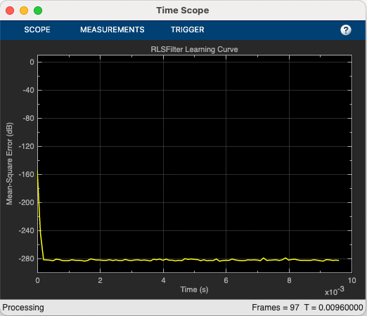
The fast convergence of the RLS filter towards the FIR filter can be seen through the above plots.

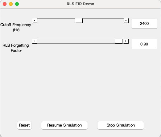
RLSFilterSystemIDExampleApp launches a User Interface (UI) designed to interact with the simulation. The UI allows you to tune parameters and the results are reflected in the simulation instantly. For example, moving the slider for the 'Cutoff Frequency' to the right while the simulation is running, increases the FIR filter's cutoff frequency. Similarly, moving the slider for the 'RLS Forgetting Factor' tunes the forgetting factor of the RLS filter. The plots reflects your changes as you tune these parameters. For more information on the UI, please refer toHelperCreateParamTuningUI.

There are also two buttons on the UI - the 'Reset' button resets the states of the RLS and FIR filters to their initial values, and 'Stop simulation' ends the simulation. If you tune the RLS filter's forgetting factor to a value that is too low, you will notice that the RLS filter fails to converge to the desired solution, as expected. You can restore convergence by first increasing the forgetting factor to an acceptable value, and then clicking the 'Reset' button. Use the UI to control either the simulation or, optionally, a MEX-file (or standalone executable) generated from the simulation code as detailed below. If you have a MIDI controller, it is possible to synchronize it with the UI. You can do this by choosing a MIDI control in the dialog that is opened when you right-click on the sliders or buttons and select "Synchronize" from the context menu. The chosen MIDI control then works in accordance with the slider/button so that operating one control is tracked by the other.

Generating the MEX-File

MATLAB Coder can be used to generate C code for the functionHelperRLSFilterSystemIdentificationSim也为了生成一个MEX-file为你platform, execute the following:

currDir = pwd;% Store the current directory addressaddpath(pwd) mexDir = [tempdir'RLSFilterSystemIdentificationExampleMEXDir'];% Name of% temporary directoryif~exist(mexDir,'dir') mkdir(mexDir);％创建临时目录endcd(mexDir);% Change directoryParamStruct = HelperRLSCodeGeneration();

Code generation successful: To view the report, open('codegen/mex/HelperRLSFilterSystemIdentificationSim/html/report.mldatx')

By calling the wrapper functionRLSFilterSystemIDExampleAppwith'true'as an argument, the generated MEX-fileHelperRLSFilterSystemIdentificationSimMEXcan be used instead ofHelperRLSFilterSystemIdentificationSimfor the simulation. In this scenario, the UI is still running inside the MATLAB environment, but the main processing algorithm is being performed by a MEX-file. Performance is improved in this mode without compromising the ability to tune parameters.

Click hereto callRLSFilterSystemIDExampleAppwith'true'as argument to use the MEX-file for simulation. Again, the simulation runs till the user explicitly stops it from the UI.

模拟与MEX速度比较

Creating MEX-Files often helps achieve faster run-times for simulations. In order to measure the performance improvement, let's first time the execution of the algorithm in MATLAB without any plotting:

clearHelperRLSFilterSystemIdentificationSimdisp('Running the MATLAB code...')

Running the MATLAB code...

tic nTimeSteps = 100;forind = 1:nTimeSteps HelperRLSFilterSystemIdentificationSim(ParamStruct);endtMATLAB = toc;

Now let's time the run of the corresponding MEX-file and display the results:

clearHelperRLSFilterSystemIdentificationSimdisp('Running the MEX-File...')

Running the MEX-File...

ticforind = 1:nTimeSteps HelperRLSFilterSystemIdentificationSimMEX(ParamStruct);endtMEX = toc; disp('RESULTS:')

RESULTS:

disp(['Time taken to run the MATLAB System object: ', num2str(tMATLAB),...' seconds']);

Time taken to run the MATLAB System object: 7.095 seconds

disp(['Time taken to run the MEX-File: ', num2str(tMEX),' seconds']);

Time taken to run the MEX-File: 0.96606 seconds

disp(['Speed-up by a factor of ', num2str(tMATLAB/tMEX),...' is achieved by creating the MEX-File']);

Speed-up by a factor of 7.3443 is achieved by creating the MEX-File

Clean up Generated Files

The temporary directory previously created can be deleted through:

cd(currDir); clearHelperRLSFilterSystemIdentificationSimMEX; rmdir(mexDir,'s');

Simulink Version

rlsfiltersystemidentificationis a Simulink model that implements the RLS System identification example highlighted in the previous sections.

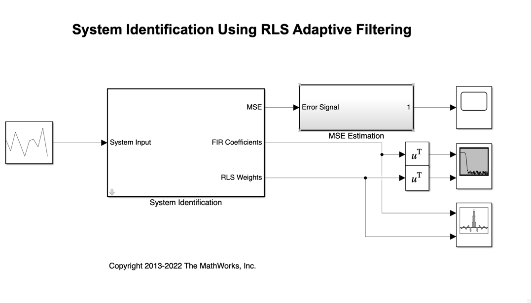
In this model, the lowpass FIR filter is modeled using theVariable Bandwidth FIR Filterblock. Magnitude response visualization is performed usingdsp.DynamicFilterVisualizer.

Double-clickthe System Identification subsystemto launch the mask designed to interact with the Simulink model. You can tune the cutoff frequency of the FIR filter and the forgetting factor of the RLS filter.

模型模拟时会生成代码。因此，必须从具有写入权限的文件夹中执行它。