Air Traffic Control

Open Live Script

This example shows how to generate an air traffic control scenario, simulate radar detections from an airport surveillance radar (ASR), and configure a global nearest neighbor (GNN) tracker to track the simulated targets using the radar detections. This enables you to evaluate different target scenarios, radar requirements, and tracker configurations without needing access to costly aircraft or equipment. This example covers the entire synthetic data workflow.

Air Traffic Control Scenario

Simulate an air traffic control (ATC) tower and moving targets in the scenario asplatforms. Simulation of the motion of the platforms in the scenario is managed bytrackingScenario.

Create atrackingScenarioand add the ATC tower to the scenario.

% Create tracking scenarioscenario = trackingScenario;% Add a stationary platform to model the ATC towertower = platform(scenario);

Airport Surveillance Radar

Add an airport surveillance radar (ASR) to the ATC tower. A typical ATC tower has a radar mounted 15 meters above the ground. This radar scans mechanically in azimuth at a fixed rate to provide 360 degree coverage in the vicinity of the ATC tower. Common specifications for an ASR are listed:

Sensitivity: 0 dBsm @ 111 km
Mechanical Scan: Azimuth only
Mechanical Scan Rate: 12.5 RPM
Electronic Scan: None
Field of View: 1.4 deg azimuth, 10 deg elevation
Azimuth Resolution: 1.4 deg
Range Resolution: 135 m

Model the ASR with the above specifications using thefusionRadarSensor.

rpm = 12.5; fov = [1.4;10]; scanrate = rpm*360/60;% deg/supdaterate = scanrate/fov(1);% Hzradar = fusionRadarSensor(1,'Rotator',...'UpdateRate', updaterate,...% Hz'FieldOfView', fov,...% [az;el] deg'MaxAzimuthScanRate', scanrate,...% deg/sec'AzimuthResolution', fov(1),...% deg'ReferenceRange', 111e3,...% m'ReferenceRCS', 0,...% dBsm'RangeResolution', 135,...% m'HasINS', true,...'DetectionCoordinates','Scenario');% Mount radar at the top of the tower雷达。MountingLocation = [0 0 -15]; tower.Sensors = radar;

Tilt the radar so that it surveys a region beginning at 2 degrees above the horizon. To do this, enable elevation and set the mechanical scan limits to span the radar's elevation field of view beginning at 2 degrees above the horizon. BecausetrackingScenario使用了没有rth-East-Down (NED) coordinate frame, negative elevations correspond to points above the horizon.

% Enable elevation scanning雷达。HasElevation = true;% Set mechanical elevation scan to begin at 2 degrees above the horizonelFov = fov(2); tilt = 2;% deg雷达。MechanicalElevationLimits = [-fov(2) 0]-tilt;% deg

Set the elevation field of view to be slightly larger than the elevation spanned by the scan limits. This prevents raster scanning in elevation and tilts the radar to point in the middle of the elevation scan limits.

雷达。FieldOfView(2) = elFov+1e-3;

ThefusionRadarSensormodels range and elevation bias due to atmospheric refraction. These biases become more pronounced at lower altitudes and for targets at long ranges. Because the index of refraction changes (decreases) with altitude, the radar signals propagate along a curved path. This results in the radar observing targets at altitudes which are higher than their true altitude and at ranges beyond their line-of-sight range.

Add three airliners within the ATC control sector. One airliner approaches the ATC from a long range, another departs, and the third is flying tangential to the tower. Model the motion of these airliners over a 60 second interval.

trackingScenario使用了没有rth-East-Down (NED) coordinate frame. When defining the waypoints for the airliners below, the z-coordinate corresponds to down, so heights above the ground are set to negative values.

% Duration of scenariosceneDuration = 60;% s% Inbound airlinerht = 3e3; spd = 900*1e3/3600;% m/swp = [-5e3 -40e3 -ht;-5e3 -40e3+spd*sceneDuration -ht]; traj = waypointTrajectory('Waypoints',wp,'TimeOfArrival',[0 sceneDuration]); platform(scenario,'Trajectory', traj);% Outbound airlinerht = 4e3; spd = 700*1e3/3600;% m/swp = [20e3 10e3 -ht;20e3+spd*sceneDuration 10e3 -ht]; traj = waypointTrajectory('Waypoints',wp,'TimeOfArrival',[0 sceneDuration]); platform(scenario,'Trajectory', traj);% Tangential airlinerht = 4e3; spd = 300*1e3/3600;% m/swp = [-20e3 -spd*sceneDuration/2 -ht;-20e3 spd*sceneDuration/2 -ht]; traj = waypointTrajectory('Waypoints',wp,'TimeOfArrival',[0 sceneDuration]); platform(scenario,'Trajectory', traj);

GNN Tracker

Create atrackerGNNto form tracks from the radar detections generated from the three airliners. Update the tracker with the detections generated after the completion of a full 360 degree scan in azimuth.

The tracker uses theinitFiltersupporting function to initialize a constant velocity extended Kalman filter for each new track.initFiltermodifies the filter returned byinitcvekfto match the target velocities and tracker update interval.

tracker = trackerGNN(...'Assignment','Auction',...'AssignmentThreshold',50,...'FilterInitializationFcn',@initFilter);

Visualize on a Map

You usetrackingGlobeViewerto visualize the results on top of a map display. You position the origin of the local North-East-Down (NED) coordinate system used by the tower radar and tracker at the position of Logan airport in Boston. The origin is located at 42.36306 latitude and -71.00639 longitude and 50 meters above the sea level.

origin = [42.366978, -71.022362, 50]; mapViewer = trackingGlobeViewer('ReferenceLocation',origin,...'Basemap','streets-dark'); campos(mapViewer, origin + [0 0 1e5]); drawnow; plotScenario(mapViewer,scenario); snapshot(mapViewer);

Simulate and Track Airliners

The following loop advances the platform positions until the end of the scenario has been reached. For each step forward in the scenario, the radar generates detections from targets in its field of view. The tracker is updated with these detections after the radar has completed a 360 degree scan in azimuth.

% Set simulation to advance at the update rate of the radarscenario.UpdateRate = radar.UpdateRate;% Create a buffer to collect the detections from a full scan of the radarscanBuffer = {};% Initialize the track arraytracks = objectTrack.empty;% Save visualization snapshots for each scanallsnaps = {}; scanCount = 0;%设置随机种子可重复的结果s = rng; rng(2020)whileadvance(scenario)% Update airliner positionsplotPlatform(mapViewer, scenario.Platforms([2 3 4]),'TrajectoryMode','Full');% Generate detections on targets in the radar's current field of view[dets,config] = detect(scenario); scanBuffer = [scanBuffer;dets];%#ok% Plot beam and detectionsplotCoverage(mapViewer,coverageConfig(scenario)) plotDetection(mapViewer,scanBuffer);% Update tracks when a 360 degree scan is completesimTime = scenario.SimulationTime; isScanDone = config.IsScanDone;ifisScanDone scanCount = scanCount+1;% Update tracker[tracks,~,~,info] = tracker(scanBuffer,simTime);% Clear scan buffer for next scanscanBuffer = {};elseifisLocked(tracker)% Predict tracks to the current simulation timetracks = predictTracksToTime(tracker,'confirmed',simTime);end% Update map and take snapshotsallsnaps = snapPlotTrack(mapViewer,tracks,isScanDone, scanCount, allsnaps);endallsnaps = [allsnaps, {snapshot(mapViewer)}];

Show the first snapshot taken at the completion of the radar's second scan.

figure imshow(allsnaps{1});

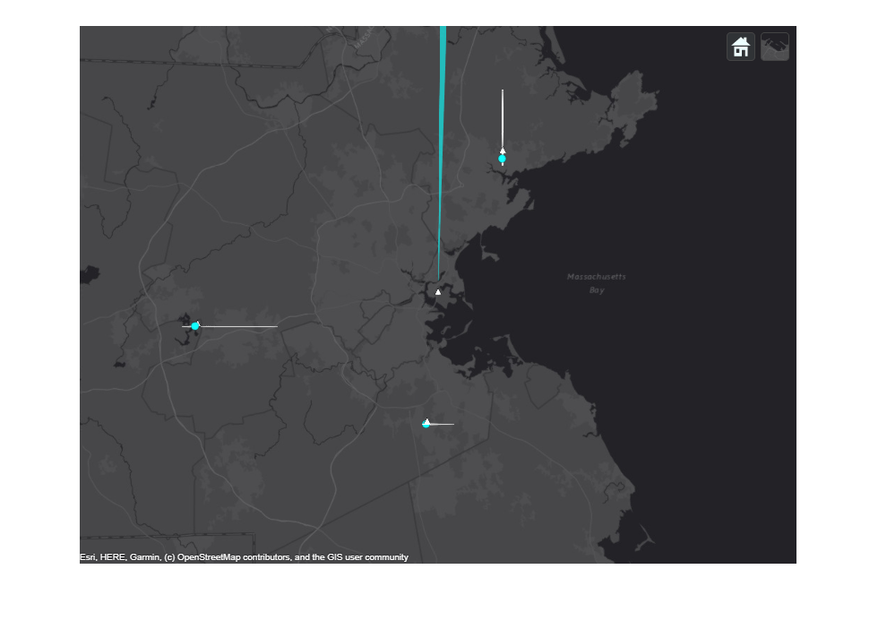
前面的图显示了最后的场景of the radar's second 360 degree scan. Radar detections, shown as light blue dots, are present for each of the simulated airliners. At this point, the tracker has already been updated by one complete scan of the radar. Internally, the tracker has initialized tracks for each of the airliners. These tracks will be shown after the update following this scan, when the tracks are promoted to confirmed, meeting the tracker's confirmation requirement of 2 hits out of 3 updates.

The next two snapshots show tracking of the outbound airliner.

figure imshow(allsnaps{2});

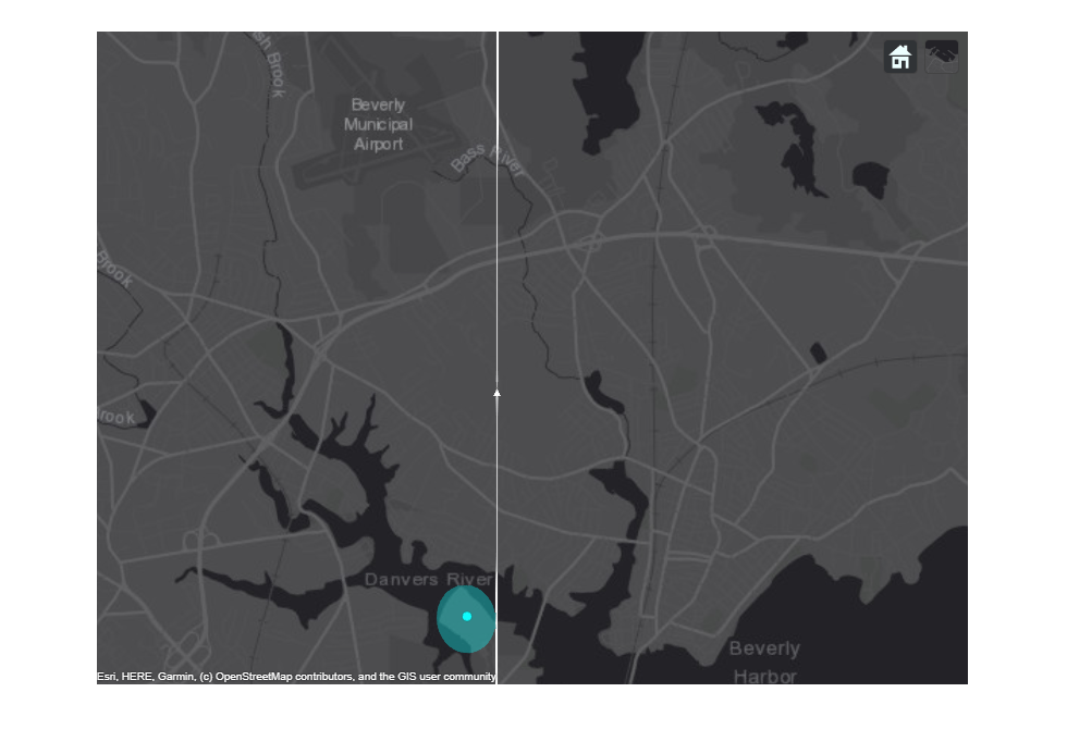
figure imshow(allsnaps{3});

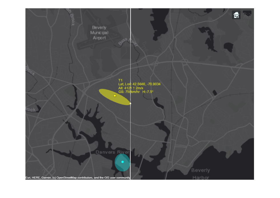
The previous figures show the track picture before and immediately after the tracker updates after the radar's second scan. The detection in the figure before the tracker update is used to update and confirm the initialized track from the previous scan's detection for this airliner. The next figure shows the confirmed track's position and velocity. The uncertainty of the track's position estimate is shown as the yellow ellipse. After only two detections, the tracker has established an accurate estimate of the outbound airliner's position and velocity. The airliner's true altitude is 4 km and it is traveling north at 700 km/hr.

figure imshow(allsnaps{4});

figure imshow(allsnaps{5});

The state of the outbound airliner's track is coasted to the end of the third scan and shown in the figure above along with the most recent detection for the airliner. Notice how the track's uncertainty has grown since it was updated in the previous figure. The track after it has been updated with the detection is shown in the next figure. You notice that the uncertainty of the track position is reduced after the update. The track uncertainty grows between updates and is reduced whenever it is updated with a new measurement. You also observe that after the third update, the track lies on top of the airliner's true position.

figure imshow(allsnaps{6});

The final figure shows the state of all three airliners' tracks at the end of the scenario. There is exactly one track for each of the three airliners. The same track numbers are assigned to each of the airliners for the entire duration of the scenario, indicating that none of these tracks were dropped during the scenario. The estimated tracks closely match the true position and velocity of the airliners.

truthTrackTable = tabulateData(scenario, tracks)%#ok

truthTrackTable=3×4 tableTrackID Altitude Heading Speed True Estimated True Estimated True Estimated _______ _________________ _________________ _________________ "T1" 4000 4051 90 90 700 710 "T2" 4000 4070 0 359 300 300 "T3" 3000 3057 0 359 900 908

Visualize tracks in 3D to get a better sense of the estimated altitudes.

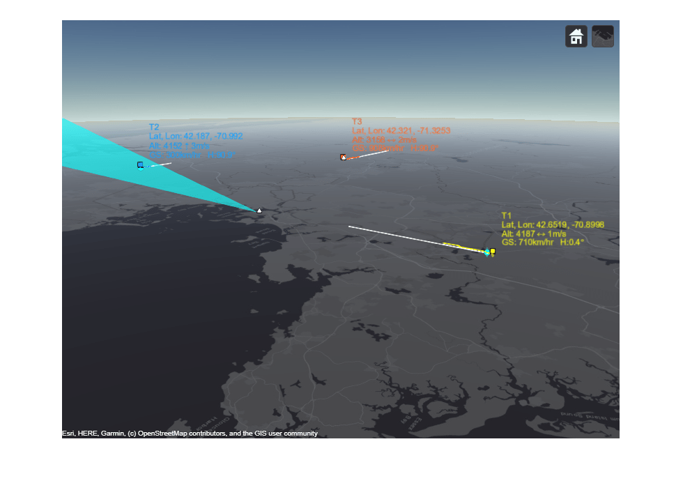
% Reposition and orient the camera to show the 3-D nature of the mapcamPosition = origin + [0.367, 0.495, 1.5e4]; camOrientation = [235, -17, 0];% Looking south west, 17 degrees below the horizoncampos(mapViewer, camPosition); camorient(mapViewer, camOrientation); drawnow

The figure below shows a 3-D map of the scenario. You can see the simulated jets in white triangles with their trajectories depicted as white lines. The radar beam is shown as a blue cone with blue dots representing radar detections. The tracks are shown in yellow, orange, and blue and their information is listed in their respective color. Due to the nature of the 3-D display, some of the markers may be hidden behind others.

You can use the following controls on the map to get different views of the scene:

To pan the map, you left click on the mouse and drag the map.
To rotate the map, while holding the ctrl button, you left click on the mouse and drag the map.
To zoom the map in and out, you use the mouse scroll wheel.

snapshot(mapViewer);

Summary

This example shows how to generate an air traffic control scenario, simulate radar detections from an airport surveillance radar (ASR), and configure a global nearest neighbor (GNN) tracker to track the simulated targets using the radar detections. In this example, you learned how the tracker's history based logic promotes tracks. You also learned how the track uncertainty grows when a track is coasted and is reduced when the track is updated by a new detection.

Supporting Functions

initFilter

This function modifies the functioninitcvekfto handle higher velocity targets such as the airliners in the ATC scenario.

functionfilter = initFilter(detection) filter = initcvekf(detection); classToUse = class(filter.StateCovariance);% Airliners can move at speeds around 900 km/h. The velocity is% initialized to 0, but will need to be able to quickly adapt to% aircraft moving at these speeds. Use 900 km/h as 1 standard deviation% for the initialized track's velocity noise.spd = 900*1e3/3600;% m/svelCov = cast(spd^2,classToUse); cov = filter.StateCovariance; cov(2,2) = velCov; cov(4,4) = velCov; filter.StateCovariance = cov;% Set filter's process noise to match filter's update ratescaleAccelHorz = cast(1,classToUse); scaleAccelVert = cast(1,classToUse); Q = blkdiag(scaleAccelHorz^2, scaleAccelHorz^2, scaleAccelVert^2); filter.ProcessNoise = Q;end

tabulateData

This function returns a table comparing the ground truth and tracks

functiontruthTrackTable = tabulateData(scenario, tracks)% Process truth dataplatforms = scenario.Platforms(2:end);% Platform 1 is the radarnumPlats = numel(platforms); trueAlt = zeros(numPlats,1); trueSpd = zeros(numPlats,1); trueHea = zeros(numPlats,1);fori = 1:numPlats traj = platforms{i}.Trajectory; waypoints = traj.Waypoints; times = traj.TimeOfArrival; trueAlt(i) = -waypoints(end,3); trueVel = (waypoints(end,:) - waypoints(end-1,:)) / (times(end)-times(end-1)); trueSpd(i) = norm(trueVel) * 3600 / 1000;% Convert to km/htrueHea(i) = atan2d(trueVel(1),trueVel(2));endtrueHea = mod(trueHea,360);% Associate tracks with targets丙氨酸= [tracks.ObjectAttributes];tgtInds =[丙氨酸。TargetIndex];% Process tracks assuming a constant velocity modelnumTrks = numel(tracks); estAlt = zeros(numTrks,1); estSpd = zeros(numTrks,1); estHea = zeros(numTrks,1); truthTrack = zeros(numTrks,7);fori = 1:numTrks estAlt(i) = -round(tracks(i).State(5)); estSpd(i) = round(norm(tracks(i).State(2:2:6)) * 3600 / 1000);% Convert to km/h;estHea(i) = round(atan2d(tracks(i).State(2),tracks(i).State(4))); estHea(i) = mod(estHea(i),360); platID = tgtInds(i); platInd = platID - 1; truthTrack(i,:) = [tracks(i).TrackID, trueAlt(platInd), estAlt(i), trueHea(platInd), estHea(i),...trueSpd(platInd), estSpd(i)];end% Organize the data in a tablenames = {'TrackID','TrueAlt','EstimatedAlt','TrueHea','EstimatedHea','TrueSpd','EstimatedSpd'}; truthTrackTable = array2table(truthTrack,'VariableNames',names); truthTrackTable = mergevars(truthTrackTable, (6:7),'NewVariableName','Speed','MergeAsTable', true); truthTrackTable.(6).Properties.VariableNames = {'True','Estimated'}; truthTrackTable = mergevars(truthTrackTable, (4:5),'NewVariableName','Heading','MergeAsTable', true); truthTrackTable.(4).Properties.VariableNames = {'True','Estimated'}; truthTrackTable = mergevars(truthTrackTable, (2:3),'NewVariableName','Altitude','MergeAsTable', true); truthTrackTable.(2).Properties.VariableNames = {'True','Estimated'}; truthTrackTable.TrackID ="T"+ string(truthTrackTable.TrackID);end

snapPlotTrack

This function handles moving the camera, taking relevant snapshots and updating track visuals.

functionallsnaps = snapPlotTrack(mapViewer,tracks,isScanDone, scanCount,allsnaps)% Save snapshots during first 4 scansifisScanDone && any(scanCount == [2 3]) newsnap = snapshot(mapViewer); allsnaps = [allsnaps, {newsnap}];%move cameraifscanCount == 2% Show the outbound airlinercampos(mapViewer, [42.5650 -70.8990 7e3]); drawnow newsnap = snapshot(mapViewer); allsnaps = [allsnaps, {newsnap}];endend% Update display with current track positionsplotTrack(mapViewer,tracks,'LabelStyle','ATC');ifisScanDone && any(scanCount == [2 3])% Take a snapshot of confirmed trackdrawnow newsnap = snapshot(mapViewer); allsnaps = [allsnaps, {newsnap}];% Reset Camera view to full sceneifscanCount == 3 origin = [42.366978, -71.022362, 50]; campos(mapViewer, origin + [0 0 1e5]); drawnowendendend