Load Earthquake Data

The filequake.matcontains 200Hz data from the October 17, 1989 Loma Prieta earthquake in the Santa Cruz Mountains. The data are courtesy of Joel Yellin at the Charles F. Richter Seismological Laboratory, University of California, Santa Cruz.

Start by loading the data.

loadquake谁是env

Name Size Bytes Class Attributes e 10001x1 80008 double n 10001x1 80008 double v 10001x1 80008 double

In the workspace there are three variables, containing time traces from an accelerometer located in the Natural Sciences building at UC Santa Cruz. The accelerometer recorded the main shock amplitude of the earthquake wave. The variablesn,e,vrefer to the three directional components measured by the instrument, which was aligned parallel to the fault, with its N direction pointing in the direction of Sacramento. The data are uncorrected for the response of the instrument.

Create a variable,Time, containing the timestamps sampled at 200Hz with the same length as the other vectors. Represent the correct units with theseconds功能和multiplication to achieve the Hz ( ${\mathit{s}}^{-1}$) sampling rate. This results in adurationvariable which is useful for representing elapsed time.

时间=（1/200）*秒（1：长度（e））';谁是Time

Name Size Bytes Class Attributes Time 10001x1 80010 duration

Organize Data in Timetable

可以在table或者timetablefor more convenience. Atimetableprovides flexibility and functionality for working with time-stamped data. Create atimetablewith the time and three acceleration variables and supply more meaningful variable names. Display the first eight rows using the头功能。

varNames = {'东西','NorthSouth','Vertical'}; quakeData = timetable(Time, e, n, v,'VariableNames', varNames); head(quakeData)

ans=8×3 timetable时间东北北部垂直_________ __________________________________ 0.005秒5 3 0 0.01 sec 5 3 0 0.015 sec 5 2 0 0.02 sec 5 2 0 0.025 sec 5 2 0 0.03 sec 5 2 0 0.035 0 0.035 sec 5 1 0 0.04 sec 5 1 0 0.04 sec 5 1 0 0 0.04 sec 5 1 0 0 0 0.04 sec 5 1 0 0

Explore the data by accessing the variables in thetimetablewith dot subscripting. (For more information on dot subscripting, seeAccess Data in a Table。) We chose "East-West" amplitude andplotit as function of the duration.

plot(quakeData.Time,quakeData.EastWest) title(“东西向加速”)

Scale Data

Scale the data by the gravitational acceleration, or multiply each variable in the table by the constant. Since the variables are all of the same type (double), you can access all variables using the dimension name,变量。注意quakeData.Variablesprovides a direct way to modify the numerical values within the timetable.

quakeData.Variables = 0.098*quakeData.Variables;

Select Subset of Data for Exploration

We are interested in the time region where the amplitude of the shockwave starts to increase from near zero to maximum levels. Visual inspection of the above plot shows that the time interval from 8 to 15 seconds is of interest. For better visualization we draw black lines at the selected time spots to draw attention to that interval. All subsequent calculations will involve this interval.

t1 = seconds(8)*[1;1]; t2 = seconds(15)*[1;1]; hold上plot([t1 t2],ylim,'K','LineWidth',2) holdoff

Store Data of Interest

Create anothertimetablewith data in this interval. Use时间范围to select the rows of interest.

tr = timerange(seconds(8),seconds(15)); dataOfInterest = quakeData(tr,:); head(dataOfInterest)

ans=8×3 timetableTime EastWest NorthSouth Vertical _________ ________ __________ ________ 8 sec -0.098 2.254 5.88 8.005 sec 0 2.254 3.332 8.01 sec -2.058 2.352 -0.392 8.015 sec -4.018 2.352 -4.116 8.02 sec -6.076 2.45 -7.742 8.025 sec -8.036 2.548 -11.466 8.03 sec -10.094 2.548 -9.8 8.035 sec -8.232 2.646 -8.134

Visualize the three acceleration variables on three separate axes.

figure subplot(3,1,1) plot(dataOfInterest.Time,dataOfInterest.EastWest) ylabel('East-West') title('Acceleration') subplot(3,1,2) plot(dataOfInterest.Time,dataOfInterest.NorthSouth) ylabel('North-South') subplot(3,1,3) plot(dataOfInterest.Time,dataOfInterest.Vertical) ylabel('Vertical')

Calculate Summary Statistics

To display statistical information about the data we use thesummary功能。

summary(dataOfInterest)

RowTimes: Time: 1400x1 duration Values: Min 8 sec Median 11.498 sec Max 14.995 sec TimeStep 0.005 sec Variables: EastWest: 1400x1 double Values: Min -255.09 Median -0.098 Max 244.51 NorthSouth: 1400x1 double Values: Min -198.55 Median 1.078 Max 204.33 Vertical: 1400x1 double Values: Min -157.88 Median 0.98 Max 134.46

Additional statistical information about the data can be calculated usingvarfun。This is useful for applying functions to each variable in a table or timetable. The function to apply is passed tovarfun作为函数句柄。下面我们应用意思是功能to all three variables and output the result in format of a table, since the time is not meaningful after computing the temporal means.

mn = varfun（@mean，dataofintest，'OutputFormat','桌子')

mn=1×3 table意思是_EastWest mean_NorthSouth mean_Vertical _____________ _______________ _____________ 0.9338 -0.10276 -0.52542

计算速度和位置

To identify the speed of propagation of the shockwave, we integrate the accelerations once. We use cumulative sums along the time variable to get the velocity of the wave front.

edot = (1/200)*cumsum(dataOfInterest.EastWest); edot = edot - mean(edot);

下面我们执行集成在所有三个变化ables to calculate the velocity. It is convenient to create a function and apply it to the variables in thetimetablewithvarfun。In this example, we included the function at the end of this file and named itVelfun。

vel = varfun（@velfun，dataofinterest）;头（vel）

ans=8×3 timetableTime velFun_EastWest velFun_NorthSouth velFun_Vertical _________ _______________ _________________ _______________ 8 sec -0.56831 0.44642 1.8173 8.005 sec -0.56831 0.45769 1.834 8.01 sec -0.5786 0.46945 1.832 8.015 sec -0.59869 0.48121 1.8114 8.02 sec -0.62907 0.49346 1.7727 8.025 sec -0.66925 0.5062 1.7154 8.03 sec -0.71972 0.51894 1.6664 8.035 sec -0.76088 0.53217 1.6257

Apply the same functionVelfun到确定位置的速度。

pos = varfun(@velFun,vel); head(pos)

ans=8×3 timetableTime velFun_velFun_EastWest velFun_velFun_NorthSouth velFun_velFun_Vertical _________ ______________________ ________________________ ______________________ 8 sec 2.1189 -2.1793 -3.0821 8.005 sec 2.1161 -2.177 -3.0729 8.01 sec 2.1132 -2.1746 -3.0638 8.015 sec 2.1102 -2.1722 -3.0547 8.02 sec 2.107 -2.1698 -3.0458 8.025 sec 2.1037 -2.1672 -3.03738.03 SEC 2.1001 -2.1646 -3.0289 8.035 SEC 2.0963 -2.162 -3.0208

没有tice how the variable names in the timetable created byvarfuninclude the name of the function used. It is useful to track the operations that have been performed on the original data. Adjust the variable names back to their original values using dot notation.

pos.properties.variablenames = varnames;

在下面，我们绘制了感兴趣的时间间隔的速度和位置的3个组成部分。

figure subplot(2,1,1) plot(vel.Time,vel.Variables) legend(quakeData.Properties.VariableNames,'地点','NorthWest') title('Velocity') subplot(2,1,2) plot(vel.Time,pos.Variables) legend(quakeData.Properties.VariableNames,'地点','NorthWest') title('位置')

可视化轨迹

The trajectories can be plotted in 2D or 3D by using the component value. In the following we will show different ways of visualizing this data.

Begin with 2-dimensional projections. Here is the first with a few values of time annotated.

figure plot(pos.NorthSouth,pos.Vertical) xlabel('North-South'）ylabel（'Vertical')% Select locations and labelnt = ceil((max(pos.Time) - min(pos.Time))/6); idx = find(fix(pos.Time/nt) == (pos.Time/nt))'; text(pos.NorthSouth(idx),pos.Vertical(idx),char(pos.Time(idx)))

Useplotmatrixto visualize a grid of scatter plots of all variables against one another and histograms of each variable on the diagonal. The output variableAx, represents each axes in the grid and can be used to identify which axes to label usingXLABEL和ylabel。

图[s，ax] = plotmatrix（pos.variables）;forii = 1：长度（varnames）xlabel（ax（end，ii），varnames {ii}）ylabel（ax（ii，1），varnames {ii}）end

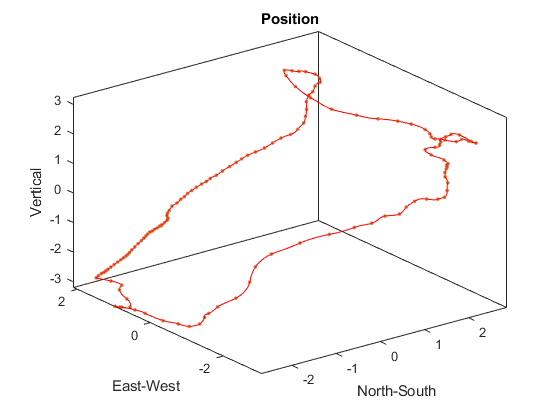
Plot a 3-D view of the trajectory and plot a dot at every tenth position point. The spacing between dots indicates the velocity.

step = 10; figure plot3(pos.NorthSouth,pos.EastWest,pos.Vertical,'r'） 抓住上plot3 (pos。没有rthSouth(1:step:end),pos.EastWest(1:step:end),pos.Vertical(1:step:end),'.'） 抓住off盒子上轴紧的Xlabel（'North-South'）ylabel（'East-West') zlabel('Vertical') title('位置')

Supporting Functions

Functions are defined below.

功能y = velFun(x) y = (1/200)*cumsum(x); y = y - mean(y);end