Modeling Cyber-Physical Systems
Cyber-physical系统结合计算机和物理al systems to achieve design goals. Simulation of cyber-physical systems requires a combination of modeling techniques such as continuous-time, discrete-time, discrete-event, and finite state modeling. Simulink® and its companion products provide functionality to apply a wide range of modeling techniques and seamlessly integrate them in one simulation environment, which is ideal for modeling cyber-physical systems.
This example shows how continuous-time, discrete-event, and finite-state modeling techniques combine to simulate the behavior of a variable speed conveyor belt system. In SimEvents®, entities are discrete items of interest in a discrete-event simulation. Because passengers are discrete individuals, they are modeled by SimEvents® entities, created by the Entity Generator block. A Stateflow® chart models the operational modes and motor dynamics of the variable speed conveyor belt. Finally, the Entity Transport Delay block models passenger throughput as a function of conveyor belt dynamics, providing a bridge between the discrete-event and continuous-time domains.
Note:The example uses blocks from SimEvents® and Stateflow®. If you do not have a SimEvents or Stateflow license, you can open and simulate the model but only make basic changes such as modifying block parameters.
Model Structure
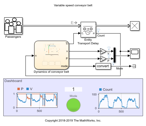
The model includes these key components:
Passengers— Models the arrival of passengers as a Poisson process. The output is a sequence of SimEvents® entities corresponding to the passengers who step on the conveyor belt. The distribution of inter-arrival time (
 ) of a Poisson process is
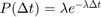 , where
 is the arrival rate.is modeled by a MATLAB action in the Entity Generator block forrush hour,normal hour, andfree hour. The passenger arrival rate changes with time as:


Entity Transport Delay— Holds the passengers on the conveyor belt until they arrive at the other terminal, based on the time delay calculated by the Stateflow chart.
Dynamics of conveyor belt— Models the operation of a variable speed conveyor belt. See theConveyor Belt Dynamicssection for more details.
Dashboard— Shows the runtime status of the conveyor belt. The color of the
ModeLamp indicates the mode of the conveyor belt.
Conveyor Belt Dynamics
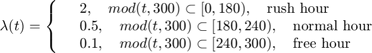
A Stateflow® chart models the dynamics of the variable speed conveyor belt. Note in the chart that the velocity and power of the belt are plotted against a logarithmic scale of the load weight. The conveyor belt has these modes:
Idle— The weight of the load is small. The belt maintains a low velocity to save energy. The
ModeLamp is gray in this mode.
OnDemand— This is the normal operating mode, which maintains the optimal velocity for passenger comfort and throughput. The power will proportionally increase with the weight of the load. The
ModeLamp is green in this mode.
Max— Maximum power mode. The weight of the load is too large for the conveyor belt to maintain the optimal velocity. The conveyor belt operates at the maximum possible velocity that does not exceed the maximum power. The
ModeLamp is red in this mode.
Results
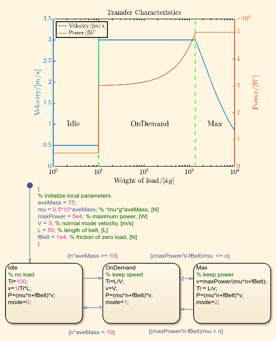
The Scope and blocks in the DashBoard show the simulation results.
Simulation results: 1. Number of passengers versus simulation time. 2. Velocity (blue) and power (red) versus simulation time.

Three operation cycles are observed within a time span of 900. Each cycle has a period of 300, which aligns with the period of the arrival rate. The top plot shows the number of passengers on the conveyor belt over time, and the bottom plot shows the velocity and power of the conveyor belt. The velocity and power are normalized for better visualization.
The first two thirds of each period correspond torush hour, and the number of passengers on the conveyor belt increases dramatically. Consequently, the conveyor belt enters into theMaxmode quickly, which is characterized by the maximum output power with a velocity that is inversely proportional to the number of passengers. In the last third of each period, the airport is in thenormal hourfollowed by thefree hour. Therefore, the number of passengers on the conveyor belt drops and even becomes zero for some time.
The conveyor belt then operates inOnDemandandIdlemodes accordingly. InOnDemandmode, the velocity is locked to a default value, and the power is proportional to the number of passengers. InIdlemode, both the velocity and power are maintained at low values to reduce energy consumption. Overall, the conveyor belt operates according to the load of the airport.
You can also select a web site from the following list:
Americas
- América Latina(Español)
- Canada(English)
- United States(English)
Europe
- Belgium(English)
- Denmark(English)
- Deutschland(Deutsch)
- España(Español)
- Finland(English)
- France(Français)
- Ireland(English)
- Italia(Italiano)
- Luxembourg(English)
- Netherlands(English)
- Norway(English)
- Österreich(Deutsch)
- Portugal(English)
- Sweden(English)
- Switzerland
- United Kingdom(English)