Reduce Model Order Using the Model Reducer App

Open Model Reducer with a Building Model

This example uses a model of the Los Angeles University Hospital building. The building has eight floors, each with three degrees of freedom: two displacements and one rotation. The input-output relationship for any one of these displacements is represented as a 48-state model, where each state represents a displacement or its rate of change (velocity). Load the building model and openModel Reducerwith that model.

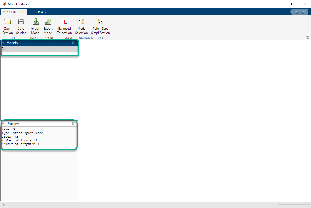
loadbuilding.matmodelReducer(G)

Select the model in the data browser to display some information about the model in the Preview section. Double-click the model to see more detailed information.

Open the Balanced Truncation Tab

Model Reducerhas three model reduction methods: Balanced Truncation, Mode Selection, and Pole/Zero Simplification. For this example, clickBalanced Truncation.

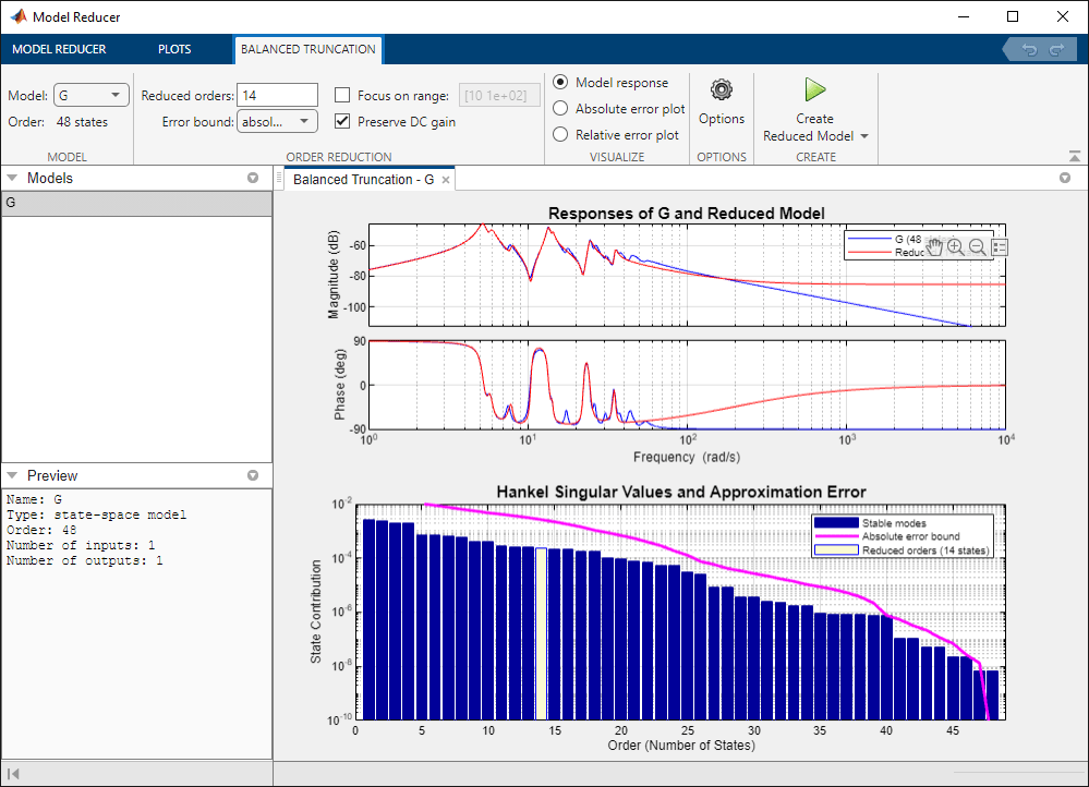
Model Reduceropens theBalanced Truncationtab and automatically generates a reduced-order model. The top plot compares the original and reduced model in the frequency domain. The bottom plot shows the energy contribution of each state, where the states are sorted from high energy to low energy. The order of the reduced model, 14, is highlighted in the bar chart. In the reduced model, all states with lower energy contribution than this one are discarded.

Compute Multiple Approximations

Suppose that you want to preserve the first, second, and third peaks of the model response, around 5.2 rad/s, 13 rad/s, and 25 rad/s. Try other model orders to see whether you can achieve this goal with a lower model order. Compute a 5th-order and a 10th-order approximation in one of the following ways:

Model Reducercomputes two new reduced-order models and displays them on the response plot with the original modelG. To examine the three peaks more closely, Zoom in on the relevant frequency range. The 10th-order model captures the three peaks successfully, while the 5th-order model only approximates the first two peaks. (For information about zooming and other interactions with the analysis plots, seeVisualize Reduced-Order Models in the Model Reducer App.)

Compare Reduced Models with Different Visualizations

In addition to the frequency response plot of all three models,Model Reducerlets you examine the absolute and relative error between the original and reduced models. SelectAbsolute error plotto see the difference between the building and reduced models.

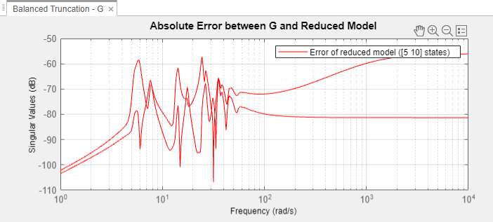
The 5th-order reduced model has at most -60dB error in the frequency region of the first two peaks, below about 30 rad/s. The error increases at higher frequencies. The 10th-order reduced model has smaller error over all frequencies.

Create Reduced Models in Data Browser

Store the reduced models in the data browser by clickingCreate Reduced Model. The 5th-order and 10th-order reduced models appear in the data browser with namesGReduced5andGreduced10.

You can continue to change the model-reduction parameters and generate additional reduced models. As you do so,GReduced5andGreduced10remain unchanged in the data browser.

Focus on Dynamics at Particular Frequencies

By default, balanced truncation inModel Reducerpreserves DC gain, matching the steady-state response of the original and reduced models. Clear thePreserve DC Gaincheckbox to better approximate high-frequency dynamics.Model Reducercomputes new reduced models. The error in the high-frequency region is decreased at the cost of a slight increase in error at low frequencies.

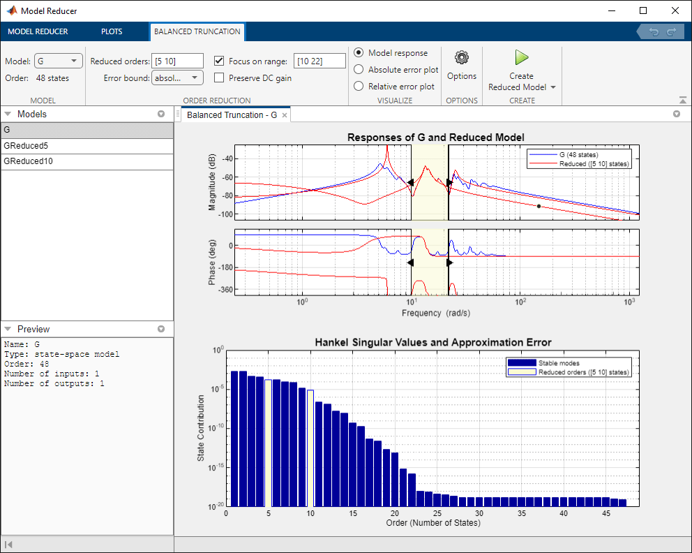
You can also focus the balanced truncation on the model dynamics in a particular frequency interval. For example, approximate only the second peak of the building model around 13 rad/s. First, select theModel responseplot to see the Bode plots of models. Then checkFocus on rangecheckbox.Model Reduceranalyzes state contributions in the highlighted frequency interval only.

You can drag the boundaries to change the frequency range interactively. As you change the frequency interval, the Hankel Singular Value plot reflects the changes in the energy contributions of the states.

Enter the frequency limits[10 22]into the text box next toFocus on range. The 5th-order reduced model captures the essential dynamics. The 10th-order model has almost the same dynamics as the original building model within this frequency range.

Optionally, store these additional models in the data browser by clickingCreate Reduced Model.

Compare Models in Time Domain

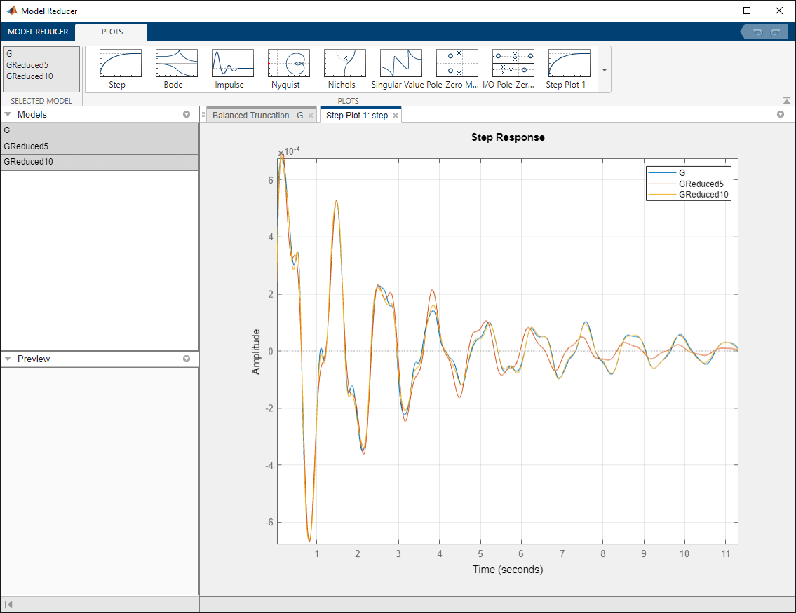
You can compare time-domain responses of the stored reduced models and the original in thePlots选项卡。在数据浏览器控件单击选择the models you want to compare,G,GReduced5, andGReduced10. Then, clickStep.Model Reducercreates a step plot with all three models.

Zooming on the transient behavior of this plot shows thatGReduced10captures the time domain behavior of the original model well. However, the response ofGReduced5deviates from the original model after about 3 seconds.

Export Model for Further Analysis

Comparison of the reduced and original models in the time and frequency domains shows thatGReduced10adequately captures the dynamics of interest. Export that model to the MATLAB® workspace for further analysis and design. In theModel Reducertab, clickExport Model. Clear the check boxes forGandGreduced5, and clickExportto exportGreduced10.

Greduced10appears in the MATLAB workspace as a state-space (ss) model.