Facility Locations

对于缩放参数的给定值 $$N$$, suppose that there are the following:

这些设施位于1和1之间的单独整数网格点上 $$N$$in the $$x$$和 $$y$$directions. In order that the facilities have separate locations, you require that $$f+w+s\le 1$$。In this example, take $$N=20$$, $$f=0。05$$, $$w=0。05$$， 和 $$s=0。1$$。

Production and Distribution

有 $$P$$products made by the factories. Take $$P=20$$。

每个产品的需求 $$p$$in a sales outlet $$s$$is $$d(s,p)$$。需求是可以在时间间隔内出售的数量。对该模型的限制是满足需求，这意味着系统会生产并精确地分配需求中的数量。

每个工厂和每个仓库都有容量限制。

Suppose that each sales outlet receives its supplies from just one warehouse. Part of the problem is to determine the cheapest mapping of sales outlets to warehouses.

费用

The cost of transporting products from factory to warehouse, and from warehouse to sales outlet, depends on the distance between the facilities, and on the particular product. If $$dist(a,b)$$是设施之间的距离 $$a$$和 $$b$$, then the cost of shipping a product $$p$$between these facilities is the distance times the transportation cost $$tcost(p)$$:

The distance in this example is the grid distance, also known as the $$L_1$$distance. It is the sum of the absolute difference in $$x$$coordinates and $$y$$coordinates.

The cost of making a unit of product $$p$$in factory $$f$$is $$pcost(f,p)$$。

优化问题

Given a set of facility locations, and the demands and capacity constraints, find:

These quantities must ensure that demand is satisfied and total cost is minimized. Also, each sales outlet is required to receive all its products from exactly one warehouse.

Variables and Equations for the Optimization Problem

控制变量（意味着您可以在优化中更改的变量）是

The objective function to minimize is

The constraints are

$$\underset{w}{\sum }x(p,f,w)\le pcap(f,p)$$（工厂的能力）。

$$\underset{f}{\sum }x(p,f,w)=\underset{s}{\sum }(d(s,p)\AA y(s,w))$$（满足需求）。

$$\underset{p}{\sum }\underset{s}{\sum }\frac{d(s,p)}{turn(p)}\AA y(s,w)\le wcap(w)$$(capacity of warehouse).

$$\underset{w}{\sum }y(s,w)=1$$（每个销售渠道都与一个仓库相关）。

$$x(p,f,w)\ge 0$$（非负生产）。

$$y(s,w)ϵ\{0,1\}$$(binary $$y$$).

变量 $$x$$和 $$y$$线性地出现在目标和约束函数中。因为 $$y$$is restricted to integer values, the problem is a mixed-integer linear program (MILP).

Generate a Random Problem: Facility Locations

Set the values of the $$N$$, $$f$$, $$w$$， 和 $$s$$参数，并生成设施位置。

RNG（1）% for reproducibilityN = 20;从10到30的％n似乎有效。谨慎选择大值。n2 = n*n;F = 0.05;工厂的密度百分比w = 0.05;% density of warehousess = 0.1;% density of sales outletsf =地板（f*n2）;% number of factoriesW =地板（w*n2）;% number of warehousesS = floor(s*N2);销售商店数量的％xyloc = randperm (N2, F + W + S);％独特的设施位置[xloc,yloc] = ind2sub([N N],xyloc);

当然，将随机位置用于设施是不现实的。此示例旨在显示解决方案技术，而不是如何生成良好的设施位置。

Plot the facilities. Facilities 1 through F are factories, F+1 through F+W are warehouses, and F+W+1 through F+W+S are sales outlets.

h = figure; plot(xloc(1:F),yloc(1:F),'rs'，xloc（f+1：f+w），yloc（f+1：f+w），'k*',...XLOC（F+W+1：F+W+S），YLOC（F+W+1：F+W+S），'bo'); lgnd = legend('工厂','Warehouse','Sales outlet','地点','EastOutside'); lgnd.AutoUpdate ='off'; xlim([0 N+1]);ylim([0 N+1])

Generate Random Capacities, Costs, and Demands

Generate random production costs, capacities, turnover rates, and demands.

p = 20;% 20 products% Production costs between 20 and 100pcost = 80*rand(F,P) + 20;% Production capacity between 500 and 1500 for each product/factoryPCAP = 1000*rand（f，p） + 500;% Warehouse capacity between P*400 and P*800 for each product/warehousewcap = p*400*rand（w，1） + p*400;每种产品1至3之间的产品周转率％turn = 2*rand(1,P) + 1;每种产品之间每距离5至10之间的产品运输成本％tcost = 5*rand（1，p） + 5;销售媒体的产品需求百分比在200到500之间％产品/出口d = 300*rand（s，p） + 200;

These random demands and capacities can lead to infeasible problems. In other words, sometimes the demand exceeds the production and warehouse capacity constraints. If you alter some parameters and get an infeasible problem, during solution you will get an exitflag of -2.

Generate Variables and Constraints

要开始指定问题，请生成距离阵列distfw(i,j)和distsw(i,j)。

distfw = zeros（f，w）;%分配矩阵工厂仓库的距离forII = 1：Fforjj = 1：w distfw（ii，jj）= abs（xloc（ii） -  xloc（f + jj）） + abs（yloc（ii）...- yloc(F + jj));endenddistsw = zeros(S,W);％为销售渠道距离矩阵分配矩阵距离forII = 1：Sforjj = 1:W distsw(ii,jj) = abs(xloc(F + W + ii) - xloc(F + jj))...+ abs(yloc(F + W + ii) - yloc(F + jj));endend

Create variables for the optimization problem.xrepresents the production, a continuous variable, with dimensionP-by-F-by-W。y代表销售渠道二进制分配给仓库，这是一个S-by-W多变的。

x = optimvar('x'，p，f，w，'LowerBound',0); y = optimvar('y'，s，w，'Type','integer','LowerBound',0,'UpperBound',1);

Now create the constraints. The first constraint is a capacity constraint on production.

capconstr = sum(x,3) <= pcap';

The next constraint is that the demand is met at each sales outlet.

demconstr = squeeze(sum(x,2)) == d'*y;

There is a capacity constraint at each warehouse.

warecap = sum(diag(1./turn)*(d'*y),1) <= wcap';

最后，有一个要求每个销售媒体恰好连接到一个仓库。

salesware = sum(y,2) == ones(S,1);

Create Problem and Objective

创建一个优化问题。

factoryprob = optimproblem;

目标函数有三个部分。第一部分是生产成本的总和。

objfun1 = sum(sum(sum(x,3).*(pcost'),2),1);

The second part is the sum of the transportation costs from factories to warehouses.

objfun2 = 0;forp = 1:P objfun2 = objfun2 + tcost(p)*sum(sum(squeeze(x(p,:,:)).*distfw));end

第三部分是从仓库到销售商店的运输成本的总和。

r = sum(distsw.*y,2);% r is a length s vectorv = d*(tcost(:)); objfun3 = sum(v.*r);

The objective function to minimize is the sum of the three parts.

factoryprob.Objective = objfun1 + objfun2 + objfun3;

Include the constraints in the problem.

FactoryProb.constraints.capconstr = capconstr;FactoryProb.constraints.demconstr = demConstr;FactoryProb.constraints.warecap = WARECAP;FactoryProb.constraints.salesware = salesware;

Solve the Problem

Turn off iterative display so that you don't get hundreds of lines of output. Include a plot function to monitor the solution progress.

opts = optimoptions(“ intlinprog”,'Display','off','plotfcn',@optimplotmilp);

Call the solver to find the solution.

[sol,fval,exitflag,output] = solve(factoryprob,'options',opts);

ifisempty(sol)% If the problem is infeasible or you stopped early with no solutiondisp(“求解器没有返回解决方案。”)返回% Stop the script because there is nothing to examineend

Examine the Solution

Examine the exit flag and the infeasibility of the solution.

exitflag

exitflag = OptimalSolution

infeas1 = max（max（不可行（CapConstr，sol）））））））

infeas1 = 9.0949e-13

infeas2 = max（max（不可行（DemConstr，sol））））））

infeas2 = 4.5475e-11

infeas3 = max（不可行（WARECAP，SOL））

infeas3 = 0

infeas4 = max(infeasibility(salesware,sol))

infeas4 = 1.3078e-13

围绕y解决方案的一部分是要完全值值的。要了解为什么这些变量可能不是整数完全是整数，请参见一些“整数”解决方案不是整数万博 尤文图斯。

sol.y =圆形（sol.y）;％获取整数解决方案万博 尤文图斯

每个仓库有多少销售商店？请注意，在这种情况下，某些仓库具有0个相关的插座，这意味着仓库不在最佳解决方案中使用。

outlets = sum(sol.y,1)

outlets =1×202 0 3 2 2 2 3 2 3 2 1 0 0 3 4 3 2 3 2 1

绘制每个销售渠道与其仓库之间的连接。

figure(h); hold上forii = 1：s jj = find（sol.y（ii，:)）;与II相关的仓库索引％Xsales = Xloc（F+W+II）;ysales = yloc（f+w+ii）;Xwarehouse = XLOC（F+JJ）;ywarehouse = yloc（f+jj）;if兰德（1）<.5％绘制y方向上半年plot([xsales,xsales,xwarehouse],[ysales,ywarehouse,ywarehouse],'g--')else％绘制X方向首先剩下的时间绘图（[XSALES，XWAREHOUSE，XWAREHOUSE]，[YSALES，YSALES，YWAREHOUSE]，'g--')endendhold离开title('Mapping of sales outlets to warehouses')

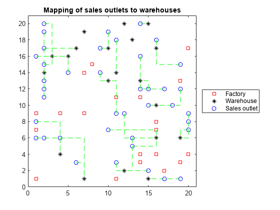
The black * with no green lines represent the unused warehouses.