Loading the Data

Load a data set comprising spectral intensities of 60 samples of gasoline at 401 wavelengths, and their octane ratings. These data are described in Kalivas, John H., "Two Data Sets of Near Infrared Spectra," Chemometrics and Intelligent Laboratory Systems, v.37 (1997) pp.255-259.

loadspectrawhos尼尔octane

Name Size Bytes Class Attributes NIR 60x401 192480 double octane 60x1 480 double

[dummy,h] = sort(octane); oldorder = get(gcf,“ DefaultaxesColorOrder”）；设置（GCF，“ DefaultaxesColorOrder”,jet(60)); plot3(repmat(1:401,60,1)',repmat(octane(h),1,401)',NIR(h,:)'); set(gcf,“ DefaultaxesColorOrder”,oldorder); xlabel('Wavelength Index'）；ylabel('Octane'）；axis('tight'）；gridon

将数据与两个组件拟合

Use theplsregressfunction to fit a PLSR model with ten PLS components and one response.

X = NIR; y = octane; [n,p] = size(X); [Xloadings,Yloadings,Xscores,Yscores,betaPLS10,PLSPctVar] = plsregress(...X,y,10);

Ten components may be more than will be needed to adequately fit the data, but diagnostics from this fit can be used to make a choice of a simpler model with fewer components. For example, one quick way to choose the number of components is to plot the percent of variance explained in the response variable as a function of the number of components.

plot(1:10,cumsum(100*PLSPctVar(2,:)),'-bo'）；xlabel('Number of PLS components'）；ylabel('Percent Variance Explained in Y'）；

In practice, more care would probably be advisable in choosing the number of components. Cross-validation, for instance, is a widely-used method that will be illustrated later in this example. For now, the above plot suggests that PLSR with two components explains most of the variance in the observedy. Compute the fitted response values for the two-component model.

[Xloadings,Yloadings,Xscores,Yscores,betaPLS] = plsregress(X,y,2); yfitPLS = [ones(n,1) X]*betaPLS;

接下来，拟合具有两个主要组件的PCR模型。第一步是对X, using thepcafunction, and retaining two principal components. PCR is then just a linear regression of the response variable on those two components. It often makes sense to normalize each variable first by its standard deviation when the variables have very different amounts of variability, however, that is not done here.

[PCALoadings,PCAScores,PCAVar] = pca(X,'Economy',false); betaPCR = regress(y-mean(y), PCAScores(:,1:2));

To make the PCR results easier to interpret in terms of the original spectral data, transform to regression coefficients for the original, uncentered variables.

betaPCR = PCALoadings(:,1:2)*betaPCR; betaPCR = [mean(y) - mean(X)*betaPCR; betaPCR]; yfitPCR = [ones(n,1) X]*betaPCR;

Plot fitted vs. observed response for the PLSR and PCR fits.

plot(y,yfitPLS,'bo',y,yfitPCR,'r^'）；xlabel('Observed Response'）；ylabel('Fitted Response'）；legend({'PLSR with 2 Components''PCR with 2 Components'},...'location','NW'）；

In a sense, the comparison in the plot above is not a fair one -- the number of components (two) was chosen by looking at how well a two-component PLSR model predicted the response, and there's no reason why the PCR model should be restricted to that same number of components. With the same number of components, however, PLSR does a much better job at fittingy. In fact, looking at the horizontal scatter of fitted values in the plot above, PCR with two components is hardly better than using a constant model. The r-squared values from the two regressions confirm that.

TSS = sum((y-mean(y)).^2); RSS_PLS = sum((y-yfitPLS).^2); rsquaredPLS = 1 - RSS_PLS/TSS

rsquaredPLS = 0.9466

RSS_PCR = sum((y-yfitPCR).^2); rsquaredPCR = 1 - RSS_PCR/TSS

rsquaredPCR = 0.1962

Another way to compare the predictive power of the two models is to plot the response variable against the two predictors in both cases.

plot3(Xscores(:,1),Xscores(:,2),y-mean(y),'bo'）；legend('PLSR'）；gridon; view(-30,30);

It's a little hard to see without being able to interactively rotate the figure, but the PLSR plot above shows points closely scattered about a plane. On the other hand, the PCR plot below shows a cloud of points with little indication of a linear relationship.

plot3(PCAScores(:,1),PCAScores(:,2),y-mean(y),'r^'）；legend('PCR'）；gridon; view(-30,30);

Notice that while the two PLS components are much better predictors of the observedy, the following figure shows that they explain somewhat less variance in the observedXthan the first two principal components used in the PCR.

plot(1:10,100*cumsum(PLSPctVar(1,:)),'b-o',1:10,...100*cumsum(PCAVar(1:10))/sum(PCAVar(1:10)),'r-^'）；xlabel('Number of Principal Components'）；ylabel(“ x中解释的百分比差异”）；legend({'PLSR''PCR'},'location','SE'）；

The fact that the PCR curve is uniformly higher suggests why PCR with two components does such a poor job, relative to PLSR, in fittingy. PCR constructs components to best explainX，结果，前两个组件忽略了数据中重要的信息，这些信息对于拟合观察到的信息很重要y.

Fitting with More Components

As more components are added in PCR, it will necessarily do a better job of fitting the original datay, simply because at some point most of the important predictive information inXwill be present in the principal components. For example, the following figure shows that the difference in residuals for the two methods is much less dramatic when using ten components than it was for two components.

yfitPLS10 = [ones(n,1) X]*betaPLS10; betaPCR10 = regress(y-mean(y), PCAScores(:,1:10)); betaPCR10 = PCALoadings(:,1:10)*betaPCR10; betaPCR10 = [mean(y) - mean(X)*betaPCR10; betaPCR10]; yfitPCR10 = [ones(n,1) X]*betaPCR10; plot(y,yfitPLS10,'bo',y,yfitPCR10,'r^'）；xlabel('Observed Response'）；ylabel('Fitted Response'）；legend({'PLSR with 10 components''PCR with 10 Components'},...'location','NW'）；

Both models fityfairly accurately, although PLSR still makes a slightly more accurate fit. However, ten components is still an arbitrarily-chosen number for either model.

Choosing the Number of Components with Cross-Validation

It's often useful to choose the number of components to minimize the expected error when predicting the response from future observations on the predictor variables. Simply using a large number of components will do a good job in fitting the current observed data, but is a strategy that leads to overfitting. Fitting the current data too well results in a model that does not generalize well to other data, and gives an overly-optimistic estimate of the expected error.

Cross-validation is a more statistically sound method for choosing the number of components in either PLSR or PCR. It avoids overfitting data by not reusing the same data to both fit a model and to estimate prediction error. Thus, the estimate of prediction error is not optimistically biased downwards.

plsregress有一个选项来估计均方预测ion error (MSEP) by cross-validation, in this case using 10-fold C-V.

[XL，YL，XS，YS，BETA，PCTVAR，PLSMSEP] = PLSREGRESS（x，y，10，10，'CV',10);

For PCR,crossvalcombined with a simple function to compute the sum of squared errors for PCR, can estimate the MSEP, again using 10-fold cross-validation.

PCRmsep = sum(crossval(@pcrsse,X,y,'KFold',10),1) / n;

PLSR的MSEP曲线表明两个或三个组件的作用尽可能出色。另一方面，PCR需要四个组件才能获得相同的预测准确性。

plot(0:10,PLSmsep(2,:),'b-o',0:10,PCRmsep,'r-^'）；xlabel('Number of components'）；ylabel('Estimated Mean Squared Prediction Error'）；legend({'PLSR''PCR'},'location','NE'）；

实际上，PCR中的第二个成分increasesthe prediction error of the model, suggesting that the combination of predictor variables contained in that component is not strongly correlated withy. Again, that's because PCR constructs components to explain variation inX, noty.

Model Parsimony

So if PCR requires four components to get the same prediction accuracy as PLSR with three components, is the PLSR model more parsimonious? That depends on what aspect of the model you consider.

The PLS weights are the linear combinations of the original variables that define the PLS components, i.e., they describe how strongly each component in the PLSR depends on the original variables, and in what direction.

[Xl,Yl,Xs,Ys,beta,pctVar,mse,stats] = plsregress(X,y,3); plot(1:401,stats.W,'-'）；xlabel('Variable'）；ylabel('PLS Weight'）；legend({'1st Component''2nd Component''3rd Component'},...'location','NW'）；

Similarly, the PCA loadings describe how strongly each component in the PCR depends on the original variables.

plot(1:401,PCALoadings(:,1:4),'-'）；xlabel('Variable'）；ylabel('PCA Loading'）；legend({'1st Component''2nd Component''3rd Component'...'4th Component'},'location','NW'）；

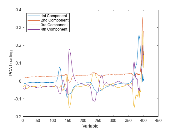
For either PLSR or PCR, it may be that each component can be given a physically meaningful interpretation by inspecting which variables it weights most heavily. For instance, with these spectral data it may be possible to interpret intensity peaks in terms of compounds present in the gasoline, and then to observe that weights for a particular component pick out a small number of those compounds. From that perspective, fewer components are simpler to interpret, and because PLSR often requires fewer components to predict the response adequately, it leads to more parsimonious models.

On the other hand, both PLSR and PCR result in one regression coefficient for each of the original predictor variables, plus an intercept. In that sense, neither is more parsimonious, because regardless of how many components are used, both models depend on all predictors. More concretely, for these data, both models need 401 spectral intensity values in order to make a prediction.

However, the ultimate goal may to reduce the original set of variables to a smaller subset still able to predict the response accurately. For example, it may be possible to use the PLS weights or the PCA loadings to select only those variables that contribute most to each component. As shown earlier, some components from a PCR model fit may serve primarily to describe the variation in the predictor variables, and may include large weights for variables that are not strongly correlated with the response. Thus, PCR can lead to retaining variables that are unnecessary for prediction.

在这个示例中,使用的数据差异in the number of components needed by PLSR and PCR for accurate prediction is not great, and the PLS weights and PCA loadings seem to pick out the same variables. That may not be true for other data.