您是否曾经想过是如何开发和原型的，在耳机，汽车和HVAC系统中发现的主动噪声消除系统是如何开发和原型的？

Let me show you a prototype using MATLAB, Simulink, and the Speedgoat Real-Time Target Machine.

Using some simple PVC pipe, this system models the type of noise cancellation system that might be used in a duct for an HVAC.

Let`s talk about how we developed this system.

The principal of active noise cancellation is that when an audio wave is summed with its exact inverse, the resulting waveform is zero.

So how does one produce a waveform that is the exact inverse of the original noise source?

当然，这不是微不足道的。但是，使用声学和信号处理的一些基本原理，我们可以设计一个系统，使我们非常令人满意的取消结果。

考虑我们的PVC管道模型的此图。我们模型中的噪声源是PVC管道一端的扬声器。消除噪声或“反噪声”来源是通过肘关节连接的另一个扬声器。

Here’s how our animation lines up with our real world PVC pipe model.

In addition to the noise and anti-noise sources, our system also uses two measurement microphones. The first measurement mic is our “reference mic”. This records the noise source close to its origin.

第二个测量麦克风称为“误差麦克风”。它放置在PVC管的输出处。该麦克风正处于发生降噪的位置。

So, if the “anti-noise” signal is just the inverse of the noise source, why can’t we just invert the reference mic signal and play that out the loud speaker? The reason is that the noise source is going to propagate down the path from its origin to the end of the pipe. We measure the audio signal at the end of the pipe with our “error microphone”. As the signal propagates, the pipe acts as a filter that changes the sound of the noise. The propagation path of the noise from its origin to the end of the tube is called the “primary path”.

我们可以使用“自适应过滤器”算法来确定此“主要路径”过滤器的特性。该过滤器将适应，直到它学习了提供此过滤器数字表示的过滤器权重。

The update algorithm that we use to update the filter weights is called “Normalized LMS”.

But wait, the anti-noise speaker has its own propagation path as well! We must also take that path into account. The propagation path from the anti-noise speaker to the error microphone is called the “secondary path”. We include an estimate of that secondary path in our system before the NLMS update.

那么，我们现在完成了吗？不完全的！要考虑的最终途径是从反噪声扬声器到噪声参考麦克风的反馈路径。我们需要从我们的参考麦克风中减去该反噪声信号，否则我们有一个连续的反馈回路，这将导致结果不正确。

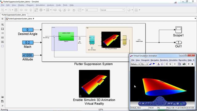
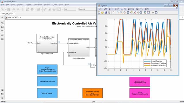
Okay, now we’re ready to simulate. Using Simulink, we created a simulated model of our real-world PVC tube system and our active-noise cancellation algorithm.

This model allows us to simulate a real-world system using a rapid prototyping environment.

For example, in this model we are simulating the primary and secondary propagation paths with digital filter equivalents. In addition, we simulate the acoustic summation of the noise and anti-noise signals with a summing block.

Now, anybody who has developed real-time audio hardware systems knows there can be inconveniences and technical difficulties that can often occur and get in the way of focusing on your algorithm. The great thing about this approach is that we can start off without hardware, test/debug the algorithm, then replace the simulated portions of our algorithm with the real-world equivalents once we’re confident it is working well.

This workflow is often referred to as model-based design.

When we run this model in simulation, we can listen in real-time to the audio signal.

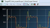
We can also view how the signals change over time on the time scope. The yellow signal represents the input noise signal, so it stays constant. The blue signal represents the signal as measured at the error microphone. When we run the simulation, we see the blue signal reduce in amplitude over time as the filter adapts.

Here we see the filter weights that are changing over time as the filter adapts.

Once we are confident our algorithm is working in simulation, the next step is to replace the simulated acoustic environment by the actual real-world system. To do this, we need a tool that will allow us to get audio signals into and out of our Simulink model with ultra-low latency.

为了实现最佳的延迟性能，我们使用Simulink实时和Speedgoat实时目标机进行了模型。万博1manbetx

This machine offers an ultra-low latency real-time kernel and ultra-low latency converters that allow signals to pass through much faster than a conventional desktop or laptop.

Why do we care about having low latency? Let’s return to our model. The system must record the reference microphone, compute the response and play it back on the ANC loudspeaker in the time it takes for sound to travel between these points. In this example, the distance between the reference microphone and the beginning of the “Y” section is 34 cm. The speed of sound is 343 m/s, thus our maximum latency is 1 ms.

The Speedgoat can be equipped with the necessary A/D and D/A converters to get the audio in and out of the machine with very low latency. In fact, with this solution the total latency is 2 samples. If we use an 8khz sampling rate, that’s a quarter of a millisecond!

我们可以通过一些简单的修改使我们万博1manbetx的Simulink模型在Speedgoat硬件上运行。

We’ll interface with the real-world audio signals going to and from our Speedgoat target machine using these custom Simulink blocks. These blocks allow us to specify things like the sample rate and voltage-range of our audio signals.

我们还可以访问“目标范围”，使我们能够可视化连接到目标机器的监视器上的信号。

Here we see the Active Noise Control portion of model, adapted to run on the Speedgoat.

Because we have used a model-based-design approach, this model is very similar to the simulation model we built for testing our algorithm originally.

We have removed the blocks that simulate our acoustic filtering and acoustic summation because they are no longer needed. We are now interfacing directly with real-world signals.

Another capability we have added to our model is a block to perform “secondary path estimation”. This allows us to replace the estimate of our secondary path that was used during simulation with an actual measurement of the real-world secondary path.

当模型首次运行时，将进行此测量。测量完成后，我们将切换到执行主动噪声消除。

We do the same thing for the acoustic feedback.

这是我们在Speedgoat机器上实时运行的模型。

We start off with the model measuring the Secondary Path Estimation and acoustic feedback. This is done by sending a white noise signal through the anti-noise speaker.

完成之后，我们切换到产生的噪音。生成的噪声源由合成的音调组成，这些调子模拟了HVAC风扇或电动机的振动。另外，我们可以使用类似噪声类型的现实录音。

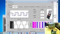
我们开始与系统。我们可以监控easurement microphone signals on our real-time scope monitor. Also, we can view the level of the noise signal with the decibel meter we have placed next to the measurement microphone.

Now, we’ll turn on the active noise control using this dashboard switch on our model.

The noise level at the decibel meter starts to decrease. Within a few seconds, we see very noticeable results. The noise has reduced by 20 db!

We hope this video has offered some helpful insight into our methodology for rapidly prototyping an active noise cancellation system with real-time streaming audio.

We were able to create a realistic model of our system using Simulink and then apply that model to real-world implementation with Simulink Real-Time and the Speedgoat Real-Time target machine.