受動性@ @ンデックス
この例は,線形時不変システムの受動性のさまざまな測定値の計算方法を示します。
受動システム
線形システムG(s)は,すべてのI/O軌跡<年代pan class="inlineequation"> が次を満たす場合に受動的です。
ここで,<年代pan class="inlineequation"> は<年代pan class="inlineequation"> の転置を表します。
システムが“どれだけ受動的であるか”を測定するために,受動性escンデックスを使用します。
入力受動性@ @ンデックスは次を満たす最大の<年代pan class="inlineequation"> として定義される
のとき,システムgは“入力で厳密に受動的”(isp)です。<年代pan class="inlineequation"> は”入力フィードフォワード受動性”(奖学金)インデックスとも呼ばれ,システムを受動的にするために必要な最小のフィードフォワードアクションに相当します。
出力受動性@ @ンデックスは次を満たす最大の<年代pan class="inlineequation"> として定義される
のとき,システムgは“出力で厳密に受動的”(osp)です。<年代pan class="inlineequation"> は”出力フィードバック受動性”(游戏)インデックスとも呼ばれ,システムを受動的にするために必要な最小のフィードバックアクションに相当します。
I/O受動性aaplンデックスは次を満たす最大の<年代pan class="inlineequation"> として定義される
のとき,システムは“非常に厳密に受動的”(vsp)です。
回路の例
次の例を考えます。電流<年代pan class="inlineequation"> を入力,電圧<年代pan class="inlineequation"> を出力とします。キルヒホッフの電圧則および電流則に基づき,<年代pan class="inlineequation"> にいて次の伝達関数を得ます。

、<年代pan class="inlineequation"> ,および<年代pan class="inlineequation"> とします。
R = 2;L = 1;C = 0.1;S = tf(<年代pan style="color:#A020F0">“年代”);G = (L*s+R)*(R*s+1/C)/(L*s^2 + 2*R*s+1/C);
isPassiveを使用して<年代pan class="inlineequation">
が受動的であるかどうかを確認します。
PF =被动(G)
PF =<年代pan class="emphasis">逻辑1
PF = trueであるため,<年代pan class="inlineequation">
は受動的です。getPassiveIndexを使用して<年代pan class="inlineequation">
の受動性@ @ンデックスを計算します。
输入被动指数nu = getPassiveIndex(G,<年代pan style="color:#A020F0">“在”)
Nu = 2
输出无源性指数rho = getPassiveIndex(G,<年代pan style="color:#A020F0">“出”)
罗= 0.2857
% I/O被动指数tau = getPassiveIndex(G,<年代pan style="color:#A020F0">“输入输出”)
Tau = 0.2642
であるため,システム<年代pan class="inlineequation"> は非常に厳密に受動的です。
周波数領域の特性
線形システムは,次のように"正の実数"である場合にのみ受動的です。
左辺の最小の固有値は,入力受動性<年代pan class="inlineequation"> に関連しています。
ここで,<年代pan class="inlineequation"> は最小の固有値を表します。同様に,<年代pan class="inlineequation"> が最小位相のとき,出力受動性。
回路の例でこれを検証します。回路の伝達関数のナ@ @キスト線図をプロットします。
尼奎斯特(G)
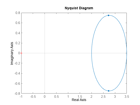
ナ电子邮箱キスト線図全体が右半平面にあるため,<年代pan class="inlineequation"> は正の実数です。ナ@ @キスト曲線で一番左の点は<年代pan class="inlineequation"> なので,入力受動性<年代pan class="inlineequation"> であり,前に取得した値と同じです。同様に,<年代pan class="inlineequation"> のナaapl . exeキスト曲線で一番左の点により,出力受動性aapl . exeンデックス値<年代pan class="inlineequation"> が与えられます。
相対受動性@ @ンデックス
次の“正の実数”条件
が,次のスモ,ルゲ,ン条件と同等であることを示せます。
相対受動性大庆市ンデックス(r大庆市ンデックス)は,<年代pan class="inlineequation"> が最小位相のとき<年代pan class="inlineequation"> の周波数にンであり,<年代pan class="inlineequation"> です。
時間領域の場合,r esc escンデックスは次を満たす最小の<年代pan class="inlineequation"> です。
システム<年代pan class="inlineequation">
は<年代pan class="inlineequation">
の場合にのみ受動的になり,<年代pan class="inlineequation">
が小さいほどシステムはより受動的になります。getPassiveIndexを使用して回路の例のr esc escンデックスを計算します。
R = getPassiveIndex(G)
R = 0.5556
結果の<年代pan class="inlineequation"> 値は,回路が極めて受動的なシステムであることを示します。
参照
[1]夏,M., P. Gahinet, N. Abroug, C. Buhr, E. Laroche。稳定性分析与控制设计中的扇形边界国际鲁棒与非线性控制杂志第30期。18(2020年12月):7857-82。https://doi.org/10.1002/rnc.5236.
参考
getPassiveIndex|<年代pan itemscope itemtype="//www.tianjin-qmedu.com/help/schema/MathWorksDocPage/SeeAlso" itemprop="seealso">isPassive
関連するトピック
您也可以从以下列表中选择一个网站: