bayesopt
Select optimal machine learning hyperparameters using Bayesian optimization
Description
attempts to find values ofresults
= bayesopt(fun
,vars
)vars
that minimizefun(vars)
.
Note
To include extra parameters in an objective function, seeParameterizing Functions.
modifies the optimization process according to theresults
= bayesopt(fun
,vars
,Name,Value
)Name,Value
arguments.
Examples
Create aBayesianOptimization
Object Usingbayesopt
This example shows how to create aBayesianOptimization
对象by usingbayesopt
to minimize cross-validation loss.
Optimize hyperparameters of a KNN classifier for theionosphere
data, that is, find KNN hyperparameters that minimize the cross-validation loss. Havebayesopt
minimize over the following hyperparameters:
Nearest-neighborhood sizes from 1 to 30
Distance functions
'chebychev'
,'euclidean'
, and'minkowski'
.
For reproducibility, set the random seed, set the partition, and set theAcquisitionFunctionName
option to'expected-improvement-plus'
. To suppress iterative display, set'Verbose'
to0
. Pass the partitionc
and fitting dataX
andY
to the objective functionfun
by creatingfun
as an anonymous function that incorporates this data. SeeParameterizing Functions.
loadionosphererngdefaultnum = optimizableVariable('n',[1,30],'Type','integer'); dst = optimizableVariable('dst',{'chebychev','euclidean','minkowski'},'Type','categorical'); c = cvpartition(351,'Kfold',5); fun = @(x)kfoldLoss(fitcknn(X,Y,'CVPartition',c,'NumNeighbors',x.n,...'Distance',char(x.dst),'NSMethod','exhaustive')); results = bayesopt(fun,[num,dst],'Verbose',0,...'AcquisitionFunctionName','expected-improvement-plus')
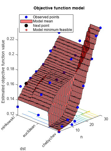
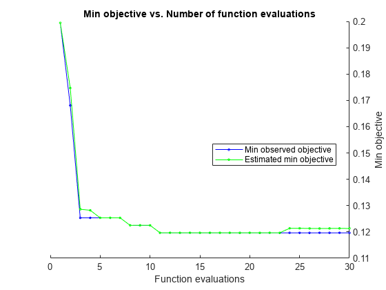
results = BayesianOptimization with properties: ObjectiveFcn: [function_handle] VariableDescriptions: [1x2 optimizableVariable] Options: [1x1 struct] MinObjective: 0.1197 XAtMinObjective: [1x2 table] MinEstimatedObjective: 0.1213 XAtMinEstimatedObjective: [1x2 table] NumObjectiveEvaluations: 30 TotalElapsedTime: 29.7824 NextPoint: [1x2 table] XTrace: [30x2 table] ObjectiveTrace: [30x1 double] ConstraintsTrace: [] UserDataTrace: {30x1 cell} ObjectiveEvaluationTimeTrace: [30x1 double] IterationTimeTrace: [30x1 double] ErrorTrace: [30x1 double] FeasibilityTrace: [30x1 logical] FeasibilityProbabilityTrace: [30x1 double] IndexOfMinimumTrace: [30x1 double] ObjectiveMinimumTrace: [30x1 double] EstimatedObjectiveMinimumTrace: [30x1 double]
Bayesian Optimization with Coupled Constraints
A coupled constraint is one that can be evaluated only by evaluating the objective function. In this case, the objective function is the cross-validated loss of an SVM model. The coupled constraint is that the number of support vectors is no more than 100. The model details are inOptimize Cross-Validated Classifier Using bayesopt.
Create the data for classification.
rngdefaultgrnpop = mvnrnd([1,0],eye(2),10); redpop = mvnrnd([0,1],eye(2),10); redpts = zeros(100,2); grnpts = redpts;fori = 1:100 grnpts(i,:) = mvnrnd(grnpop(randi(10),:),eye(2)*0.02); redpts(i,:) = mvnrnd(redpop(randi(10),:),eye(2)*0.02);endcdata = [grnpts;redpts]; grp = ones(200,1); grp(101:200) = -1; c = cvpartition(200,'KFold',10); sigma = optimizableVariable('sigma',[1e-5,1e5],'Transform','log'); box = optimizableVariable('box',[1e-5,1e5],'Transform','log');
The objective function is the cross-validation loss of the SVM model for partitionc
. The coupled constraint is the number of support vectors minus 100.5. This ensures that 100 support vectors give a negative constraint value, but 101 support vectors give a positive value. The model has 200 data points, so the coupled constraint values range from -99.5 (there is always at least one support vector) to 99.5. Positive values mean the constraint is not satisfied.
function[objective,constraint] = mysvmfun(x,cdata,grp,c) SVMModel = fitcsvm(cdata,grp,'KernelFunction','rbf',...'BoxConstraint',x.box,...'KernelScale',x.sigma); cvModel = crossval(SVMModel,'CVPartition',c); objective = kfoldLoss(cvModel); constraint = sum(SVMModel.IsSupportVector)-100.5;
Pass the partitionc
and fitting datacdata
andgrp
to the objective functionfun
by creatingfun
as an anonymous function that incorporates this data. SeeParameterizing Functions.
fun = @(x)mysvmfun(x,cdata,grp,c);
Set theNumCoupledConstraints
to1
so the optimizer knows that there is a coupled constraint. Set options to plot the constraint model.
results = bayesopt(fun,[sigma,box],'IsObjectiveDeterministic',true,...'NumCoupledConstraints',1,'PlotFcn',...{@plotMinObjective,@plotConstraintModels},...'AcquisitionFunctionName','expected-improvement-plus','Verbose',0);
Most points lead to an infeasible number of support vectors.
Parallel Bayesian Optimization
Improve the speed of a Bayesian optimization by using parallel objective function evaluation.
Prepare variables and the objective function for Bayesian optimization.
The objective function is the cross-validation error rate for the ionosphere data, a binary classification problem. Usefitcsvm
as the classifier, withBoxConstraint
andKernelScale
as the parameters to optimize.
loadionospherebox = optimizableVariable('box',[1e-4,1e3],'Transform','log'); kern = optimizableVariable('kern',[1e-4,1e3],'Transform','log'); vars = [box,kern]; fun = @(vars)kfoldLoss(fitcsvm(X,Y,'BoxConstraint',vars.box,'KernelScale',vars.kern,...'Kfold',5));
Search for the parameters that give the lowest cross-validation error by using parallel Bayesian optimization.
results = bayesopt(fun,vars,'UseParallel',true);
Copying objective function to workers... Done copying objective function to workers.
|===============================================================================================================| | Iter | Active | Eval | Objective | Objective | BestSoFar | BestSoFar | box | kern | | | workers | result | | runtime | (observed) | (estim.) | | | |===============================================================================================================| | 1 | 2 | Accept | 0.2735 | 0.56171 | 0.13105 | 0.13108 | 0.0002608 | 0.2227 | | 2 | 2 | Accept | 0.35897 | 0.4062 | 0.13105 | 0.13108 | 3.6999 | 344.01 | | 3 | 2 | Accept | 0.13675 | 0.42727 | 0.13105 | 0.13108 | 0.33594 | 0.39276 | | 4 | 2 | Accept | 0.35897 | 0.4453 | 0.13105 | 0.13108 | 0.014127 | 449.58 | | 5 | 2 | Best | 0.13105 | 0.45503 | 0.13105 | 0.13108 | 0.29713 | 1.0859 |
| 6 | 6 | Accept | 0.35897 | 0.16605 | 0.13105 | 0.13108 | 8.1878 | 256.9 |
| 7 | 5 | Best | 0.11396 | 0.51146 | 0.11396 | 0.11395 | 8.7331 | 0.7521 | | 8 | 5 | Accept | 0.14245 | 0.24943 | 0.11396 | 0.11395 | 0.0020774 | 0.022712 |
| 9 | 6 | Best | 0.10826 | 4.0711 | 0.10826 | 0.10827 | 0.0015925 | 0.0050225 |
| 10 | 6 | Accept | 0.25641 | 16.265 | 0.10826 | 0.10829 | 0.00057357 | 0.00025895 |
| 11 | 6 | Accept | 0.1339 | 15.581 | 0.10826 | 0.10829 | 1.4553 | 0.011186 |
| 12 | 6 | Accept | 0.16809 | 19.585 | 0.10826 | 0.10828 | 0.26919 | 0.00037649 |
| 13 | 6 | Accept | 0.20513 | 18.637 | 0.10826 | 0.10828 | 369.59 | 0.099122 |
| 14 | 6 | Accept | 0.12536 | 0.11382 | 0.10826 | 0.10829 | 5.7059 | 2.5642 |
| 15 | 6 |接受| 0.13675 | 2.63 | 0.10826 | 0.10828 | 984.19 | 2.2214 |
| 16 | 6 | Accept | 0.12821 | 2.0743 | 0.10826 | 0.11144 | 0.0063411 | 0.0090242 |
| 17 | 6 | Accept | 0.1339 | 0.1939 | 0.10826 | 0.11302 | 0.00010225 | 0.0076795 |
| 18 | 6 | Accept | 0.12821 | 0.20933 | 0.10826 | 0.11376 | 7.7447 | 1.2868 |
| 19 | 4 | Accept | 0.55556 | 17.564 | 0.10826 | 0.10828 | 0.0087593 | 0.00014486 | | 20 | 4 | Accept | 0.1396 | 16.473 | 0.10826 | 0.10828 | 0.054844 | 0.004479 | |===============================================================================================================| | Iter | Active | Eval | Objective | Objective | BestSoFar | BestSoFar | box | kern | | | workers | result | | runtime | (observed) | (estim.) | | | |===============================================================================================================| | 21 | 4 | Accept | 0.1339 | 0.17127 | 0.10826 | 0.10828 | 9.2668 | 1.2171 |
| 22 | 4 | Accept | 0.12821 | 0.089065 | 0.10826 | 0.10828 | 12.265 | 8.5455 |
| 23 | 4 | Accept | 0.12536 | 0.073586 | 0.10826 | 0.10828 | 1.3355 | 2.8392 |
| 24 | 4 | Accept | 0.12821 | 0.08038 | 0.10826 | 0.10828 | 131.51 | 16.878 |
| 25 | 3 | Accept | 0.11111 | 10.687 | 0.10826 | 0.10867 | 1.4795 | 0.041452 | | 26 | 3 | Accept | 0.13675 | 0.18626 | 0.10826 | 0.10867 | 2.0513 | 0.70421 |
| 27 | 6 | Accept | 0.12821 | 0.078559 | 0.10826 | 0.10868 | 980.04 | 44.19 |
| 28 | 5 | Accept | 0.33048 | 0.089844 | 0.10826 | 0.10843 | 0.41821 | 10.208 | | 29 | 5 | Accept | 0.16239 | 0.12688 | 0.10826 | 0.10843 | 172.39 | 141.43 |
| 30 | 5 | Accept | 0.11966 | 0.14597 | 0.10826 | 0.10846 | 639.15 | 14.75 |
__________________________________________________________ Optimization completed. MaxObjectiveEvaluations of 30 reached. Total function evaluations: 30 Total elapsed time: 48.2085 seconds. Total objective function evaluation time: 128.3472 Best observed feasible point: box kern _________ _________ 0.0015925 0.0050225 Observed objective function value = 0.10826 Estimated objective function value = 0.10846 Function evaluation time = 4.0711 Best estimated feasible point (according to models): box kern _________ _________ 0.0015925 0.0050225 Estimated objective function value = 0.10846 Estimated function evaluation time = 2.8307
Return the best feasible point in the Bayesian modelresults
by using thebestPoint
function. Use the default criterionmin-visited-upper-confidence-interval
, which determines the best feasible point as the visited point that minimizes an upper confidence interval on the objective function value.
zbest = bestPoint(results)
zbest=1×2 tablebox kern _________ _________ 0.0015925 0.0050225
The tablezbest
contains the optimal estimated values for the'BoxConstraint'
and'KernelScale'
name-value pair arguments. Use these values to train a new optimized classifier.
Mdl = fitcsvm(X,Y,'BoxConstraint',zbest.box,'KernelScale',zbest.kern);
Observe that the optimal parameters are inMdl
.
Mdl.BoxConstraints(1)
ans = 0.0016
Mdl.KernelParameters.Scale
ans = 0.0050
Input Arguments
fun
—Objective function
function handle|parallel.pool.Constant
whoseValue
is a function handle
Objective function, specified as a function handle or, when theUseParallel
name-value pair istrue
, aparallel.pool.Constant
(Parallel Computing Toolbox)whoseValue
is a function handle. Typically,fun
returns a measure of loss (such as a misclassification error) for a machine learning model that has tunable hyperparameters to control its training.fun
has these signatures:
对象ive = fun(x)% or[objective,constraints] = fun(x)% or[objective,constraints,UserData] = fun(x)
fun
acceptsx
, a 1-by-D
表格of variable values, and returns对象ive
, a real scalar representing the objective function valuefun(x)
.
Optionally,fun
also returns:
constraints
, a real vector of coupled constraint violations. For a definition, seeCoupled Constraints.constraint(j) > 0
means constraintj
is violated.constraint(j) < 0
means constraintj
is satisfied.UserData
, an entity of any type (such as a scalar, matrix, structure, or object). For an example of a custom plot function that usesUserData
, seeCreate a Custom Plot Function.
For details about usingparallel.pool.Constant
withbayesopt
, seePlacing the Objective Function on Workers.
Example:@objfun
Data Types:function_handle
vars
—Variable descriptions
vector ofoptimizableVariable
对象s defining the hyperparameters to be tuned
Variable descriptions, specified as a vector ofoptimizableVariable
对象s defining the hyperparameters to be tuned.
Example:[X1,X2]
, whereX1
andX2
areoptimizableVariable
对象s
Name-Value Arguments
Specify optional pairs of arguments asName1=Value1,...,NameN=ValueN
, whereName
is the argument name andValue
is the corresponding value. Name-value arguments must appear after other arguments, but the order of the pairs does not matter.
Before R2021a, use commas to separate each name and value, and encloseName
in quotes.
Example:results = bayesopt(fun,vars,'AcquisitionFunctionName','expected-improvement-plus')
AcquisitionFunctionName
—Function to choose next evaluation point
'expected-improvement-per-second-plus'
(default) |'expected-improvement'
|'expected-improvement-plus'
|'expected-improvement-per-second'
|'lower-confidence-bound'
|'probability-of-improvement'
Function to choose next evaluation point, specified as one of the listed choices.
Acquisition functions whose names includeper-second
do not yield reproducible results because the optimization depends on the runtime of the objective function. Acquisition functions whose names includeplus
modify their behavior when they are overexploiting an area. For more details, seeAcquisition Function Types.
Example:'AcquisitionFunctionName','expected-improvement-per-second'
IsObjectiveDeterministic
—Specify deterministic objective function
false
(default) |true
Specify deterministic objective function, specified asfalse
ortrue
. Iffun
is stochastic (that is,fun(x)
can return different values for the samex
), then setIsObjectiveDeterministic
tofalse
. In this case,bayesopt
estimates a noise level during optimization.
Example:'IsObjectiveDeterministic',true
Data Types:logical
ExplorationRatio
—Propensity to explore
0.5
(default) |positive real
Propensity to explore, specified as a positive real. Applies to the'expected-improvement-plus'
and'expected-improvement-per-second-plus'
acquisition functions. SeePlus.
Example:“ExplorationRatio”,0.2
Data Types:double
GPActiveSetSize
—Fit Gaussian Process model toGPActiveSetSize
or fewer points
300
(default) |positive integer
Fit Gaussian Process model toGPActiveSetSize
or fewer points, specified as a positive integer. Whenbayesopt
has visited more thanGPActiveSetSize
points, subsequent iterations that use a GP model fit the model toGPActiveSetSize
points.bayesopt
chooses points uniformly at random without replacement among visited points. Using fewer points leads to faster GP model fitting, at the expense of possibly less accurate fitting.
Example:'GPActiveSetSize',80
Data Types:double
UseParallel
—Compute in parallel
false
(default) |true
Compute in parallel, specified asfalse
(do not compute in parallel) ortrue
(compute in parallel). Computing in parallel requires Parallel Computing Toolbox™.
bayesopt
执行并行目标函数评价concurrently on parallel workers. For algorithmic details, seeParallel Bayesian Optimization.
Example:'UseParallel',true
Data Types:logical
ParallelMethod
—Imputation method for parallel worker objective function values
'clipped-model-prediction'
(default) |'model-prediction'
|'max-observed'
|'min-observed'
Imputation method for parallel worker objective function values, specified as'clipped-model-prediction'
,'model-prediction'
,'max-observed'
, or'min-observed'
. To generate a new point to evaluate,bayesopt
fits a Gaussian process to all points, including the points being evaluated on workers. To fit the process,bayesopt
imputes objective function values for the points that are currently on workers.ParallelMethod
specifies the method used for imputation.
'clipped-model-prediction'
— Impute the maximum of these quantities:Mean Gaussian process prediction at the point
x
Minimum observed objective function among feasible points visited
Minimum model prediction among all feasible points
'model-prediction'
— Impute the mean Gaussian process prediction at the pointx
.'max-observed'
— Impute the maximum observed objective function value among feasible points.'min-observed'
— Impute the minimum observed objective function value among feasible points.
Example:'ParallelMethod','max-observed'
MinWorkerUtilization
—Tolerance on number of active parallel workers
floor(0.8*Nworkers)
(default) |positive integer
Tolerance on the number of active parallel workers, specified as a positive integer. Afterbayesopt
assigns a point to evaluate, and before it computes a new point to assign, it checks whether fewer thanMinWorkerUtilization
workers are active. If so,bayesopt
分配随机点within bounds to all available workers. Otherwise,bayesopt
calculates the best point for one worker.bayesopt
creates random points much faster than fitted points, so this behavior leads to higher utilization of workers, at the cost of possibly poorer points. For details, seeParallel Bayesian Optimization.
Example:'MinWorkerUtilization',3
Data Types:double
MaxObjectiveEvaluations
—Objective function evaluation limit
30
(default) |positive integer
Objective function evaluation limit, specified as a positive integer.
Example:'MaxObjectiveEvaluations',60
Data Types:double
NumSeedPoints
—Number of initial evaluation points
4
(default) |positive integer
Number of initial evaluation points, specified as a positive integer.bayesopt
chooses these points randomly within the variable bounds, according to the setting of theTransform
setting for each variable (uniform for'none'
, logarithmically spaced for'log'
).
Example:'NumSeedPoints',10
Data Types:double
XConstraintFcn
—Deterministic constraints on variables
[]
(default) |function handle
Deterministic constraints on variables, specified as a function handle.
For details, seeDeterministic Constraints — XConstraintFcn.
Example:'XConstraintFcn',@xconstraint
Data Types:function_handle
ConditionalVariableFcn
—Conditional variable constraints
[]
(default) |function handle
Conditional variable constraints, specified as a function handle.
For details, seeConditional Constraints — ConditionalVariableFcn.
Example:'ConditionalVariableFcn',@condfun
Data Types:function_handle
NumCoupledConstraints
—Number of coupled constraints
0
(default) |positive integer
Number of coupled constraints, specified as a positive integer. For details, seeCoupled Constraints.
Note
NumCoupledConstraints
is required when you have coupled constraints.
Example:'NumCoupledConstraints',3
Data Types:double
AreCoupledConstraintsDeterministic
—Indication of whether coupled constraints are deterministic
true
for all coupled constraints(default) |logical vector
Indication of whether coupled constraints are deterministic, specified as a logical vector of lengthNumCoupledConstraints
. For details, seeCoupled Constraints.
Example:'AreCoupledConstraintsDeterministic',[true,false,true]
Data Types:logical
Verbose
—Command-line display level
1
(default) |0
|2
Command-line display level, specified as0
,1
, or2
.
0
— No command-line display.1
— At each iteration, display the iteration number, result report (see the next paragraph), objective function model, objective function evaluation time, best (lowest) observed objective function value, best (lowest) estimated objective function value, and the observed constraint values (if any). When optimizing in parallel, the display also includes a column showing the number of active workers, counted after assigning a job to the next worker.The result report for each iteration is one of the following:
Accept
— The objective function returns a finite value, and all constraints are satisfied.Best
— Constraints are satisfied, and the objective function returns the lowest value among feasible points.Error
— The objective function returns a value that is not a finite real scalar.Infeas
— At least one constraint is violated.
2
— Same as1
, adding diagnostic information such as time to select the next point, model fitting time, indication that "plus" acquisition functions declare overexploiting, and parallel workers are being assigned to random points due to low parallel utilization.
Example:'Verbose',2
Data Types:double
OutputFcn
—Function called after each iteration
{}
(default) |function handle|cell array of function handles
Function called after each iteration, specified as a function handle or cell array of function handles. An output function can halt the solver, and can perform arbitrary calculations, including creating variables or plotting. Specify several output functions using a cell array of function handles.
There are two built-in output functions:
@assignInBase
— Constructs aBayesianOptimization
instance at each iteration and assigns it to a variable in the base workspace. Choose a variable name using theSaveVariableName
name-value pair.@saveToFile
— Constructs aBayesianOptimization
instance at each iteration and saves it to a file in the current folder. Choose a file name using theSaveFileName
name-value pair.
You can write your own output functions. For details, seeBayesian Optimization Output Functions.
Example:'OutputFcn',{@saveToFile @myOutputFunction}
Data Types:cell
|function_handle
SaveFileName
—File name for the@saveToFile
output function
'BayesoptResults.mat'
(default) |character vector|string scalar
File name for the@saveToFile
output function, specified as a character vector or string scalar. The file name can include a path, such as'../optimizations/September2.mat'
.
Example:'SaveFileName','September2.mat'
Data Types:char
|string
SaveVariableName
—Variable name for the@assignInBase
output function
'BayesoptResults'
(default) |character vector|string scalar
Variable name for the@assignInBase
output function, specified as a character vector or string scalar.
Example:'SaveVariableName','September2Results'
Data Types:char
|string
PlotFcn
—Plot function called after each iteration
{@plotObjectiveModel,@plotMinObjective}
(default) |'all'
|function handle|cell array of function handles
Plot function called after each iteration, specified as'all'
, a function handle, or a cell array of function handles. A plot function can halt the solver, and can perform arbitrary calculations, including creating variables, in addition to plotting.
Specify no plot function as[]
.
'all'
calls all built-in plot functions. Specify several plot functions using a cell array of function handles.
The built-in plot functions appear in the following tables.
Model Plots — Apply When D ≤ 2 | Description |
---|---|
@plotAcquisitionFunction |
Plot the acquisition function surface. |
@plotConstraintModels |
Plot each constraint model surface. Negative values indicate feasible points. Also plot aP(feasible) surface. Also plot the error model, if it exists, which ranges from Plotted error = 2*Probability(error) – 1. |
@plotObjectiveEvaluationTimeModel |
Plot the objective function evaluation time model surface. |
@plotObjectiveModel |
Plot the |
Trace Plots — Apply to All D | Description |
---|---|
@plotObjective |
Plot each observed function value versus the number of function evaluations. |
@plotObjectiveEvaluationTime |
Plot each observed function evaluation run time versus the number of function evaluations. |
@plotMinObjective |
Plot the minimum observed and estimated function values versus the number of function evaluations. |
@plotElapsedTime |
Plot three curves: the total elapsed time of the optimization, the total function evaluation time, and the total modeling and point selection time, all versus the number of function evaluations. |
You can write your own plot functions. For details, seeBayesian Optimization Plot Functions.
Note
When there are coupled constraints, iterative display and plot functions can give counterintuitive results such as:
Aminimum objectiveplot can increase.
The optimization can declare a problem infeasible even when it showed an earlier feasible point.
The reason for this behavior is that the decision about whether a point is feasible can change as the optimization progresses.bayesopt
determines feasibility with respect to its constraint model, and this model changes asbayesopt
评估点。所以“最低目标”情节n increase when the minimal point is later deemed infeasible, and the iterative display can show a feasible point that is later deemed infeasible.
Example:'PlotFcn','all'
Data Types:char
|string
|cell
|function_handle
InitialX
—Initial evaluation points
NumSeedPoints
-by-D
random initial points within bounds(default) |N
-by-D
表格
Initial evaluation points, specified as anN
-by-D
表格, whereN
is the number of evaluation points, andD
is the number of variables.
Note
If onlyInitialX
is provided, it is interpreted as initial points to evaluate. The objective function is evaluated atInitialX
.
If any other initialization parameters are also provided,InitialX
is interpreted as prior function evaluation data. The objective function is not evaluated. Any missing values are set toNaN
.
Data Types:表格
InitialObjective
—Objective values corresponding toInitialX
[]
(default) |length-N
vector
Objective values corresponding toInitialX
, specified as a length-N
vector, whereN
is the number of evaluation points.
Example:'InitialObjective',[17;-3;-12.5]
Data Types:double
InitialConstraintViolations
—Constraint violations of coupled constraints
[]
(default) |N
-by-K
matrix
约束违反的耦合约束,规范ified as anN
-by-K
matrix, whereN
is the number of evaluation points andK
is the number of coupled constraints. For details, seeCoupled Constraints.
Data Types:double
InitialErrorValues
—Errors forInitialX
[]
(default) |length-N
vector with entries-1
or1
Errors forInitialX
, specified as a length-N
vector with entries-1
or1
, whereN
is the number of evaluation points. Specify-1
for no error, and1
for an error.
Example:'InitialErrorValues',[-1,-1,-1,-1,1]
Data Types:double
InitialUserData
—Initial data corresponding toInitialX
[]
(default) |length-N
cell vector
Initial data corresponding toInitialX
, specified as a length-N
cell vector, whereN
is the number of evaluation points.
Example:'InitialUserData',{2,3,-1}
Data Types:cell
InitialObjectiveEvaluationTimes
—Evaluation times of objective function atInitialX
[]
(default) |length-N
vector
Evaluation times of objective function atInitialX
, specified as a length-N
vector, whereN
is the number of evaluation points. Time is measured in seconds.
Data Types:double
InitialIterationTimes
—Times for the firstN
iterations
{}
(default) |length-N
vector
Times for the firstN
iterations, specified as a length-N
vector, whereN
is the number of evaluation points. Time is measured in seconds.
Data Types:double
Output Arguments
results
— Bayesian optimization results
BayesianOptimization
对象
Bayesian optimization results, returned as aBayesianOptimization
对象.
More About
Coupled Constraints
Coupled constraints are those constraints whose value comes from the objective function calculation. SeeCoupled Constraints.
Tips
Bayesian optimization is not reproducible if one of these conditions exists:
You specify an acquisition function whose name includes
per-second
, such as'expected-improvement-per-second'
. Theper-second
modifier indicates that optimization depends on the run time of the objective function. For more details, seeAcquisition Function Types.You specify to run Bayesian optimization in parallel. Due to the nonreproducibility of parallel timing, parallel Bayesian optimization does not necessarily yield reproducible results. For more details, seeParallel Bayesian Optimization.
Extended Capabilities
Automatic Parallel Support
Accelerate code by automatically running computation in parallel using Parallel Computing Toolbox™.
To run in parallel, set theUseParallel
name-value argument totrue
in the call to this function.
For more general information about parallel computing, seeRun MATLAB Functions with Automatic Parallel Support(Parallel Computing Toolbox).
Version History
Introduced in R2016b
MATLAB 명령
다음 MATLAB 명령에 해당하는 링크를 클릭했습니다.
명령을 실행하려면 MATLAB 명령 창에 입력하십시오. 웹 브라우저는 MATLAB 명령을 지원하지 않습니다.
Select a Web Site
Choose a web site to get translated content where available and see local events and offers. Based on your location, we recommend that you select:.
You can also select a web site from the following list:
How to Get Best Site Performance
Select the China site (in Chinese or English) for best site performance. Other MathWorks country sites are not optimized for visits from your location.
Americas
- América Latina(Español)
- Canada(English)
- United States(English)
Europe
- Belgium(English)
- Denmark(English)
- Deutschland(Deutsch)
- España(Español)
- Finland(English)
- France(Français)
- Ireland(English)
- Italia(Italiano)
- Luxembourg(English)
- Netherlands(English)
- Norway(English)
- Österreich(Deutsch)
- Portugal(English)
- Sweden(English)
- Switzerland
- United Kingdom(English)