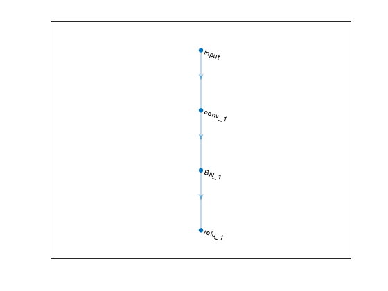
Create an empty layer graph and an array of layers. Add the layers to the layer graph and plot the graph.addLayersconnects the layers sequentially.

lgraph = layerGraph; layers = [ imageInputLayer([32 32 3],'Name','input') convolution2dLayer(3,16,'Padding','same','Name','conv_1') batchNormalizationLayer('Name','BN_1') reluLayer('Name','relu_1')]; lgraph = addLayers(lgraph,layers); figure plot(lgraph)

Create an array of layers.

layers = [ImageInputlayer（[28 28 1]，，'Name','input') convolution2dLayer(3,16,'Padding','same','Name','conv_1') batchNormalizationLayer('Name','BN_1') reluLayer('Name','relu_1')];

Create a layer graph from the layer array.layerGraphconnects all the layers inlayerssequentially. Plot the layer graph.

lgraph = layerGraph(layers); figure plot(lgraph)

Load a pretrained SqueezeNet network. You can use this trained network for classification and prediction.

net = squeezenet;

To modify the network structure, first extract the structure of the DAG network by usinglayerGraph.You can then use the object functions ofLayerGraphto modify the network architecture.

lgraph = layerGraph(net)

lgraph = LayerGraph with properties: Layers: [68x1 nnet.cnn.layer.Layer] Connections: [75x2 table] InputNames: {'data'} OutputNames: {'ClassificationLayer_predictions'}

Create a simple directed acyclic graph (DAG) network for deep learning. Train the network to classify images of digits. The simple network in this example consists of:

Create the main branch of the network as a layer array. The addition layer sums multiple inputs element-wise. Specify the number of inputs for the addition layer to sum. To easily add connections later, specify names for the first ReLU layer and the addition layer.

layers = [ imageInputLayer([28 28 1]) convolution2dLayer(5,16,'Padding','same') batchNormalizationLayer reluLayer('Name','relu_1') convolution2dLayer(3,32,'Padding','same','Stride',2) batchNormalizationLayer reluLayer convolution2dLayer(3,32,'Padding','same') batchNormalizationLayer reluLayer additionLayer(2,'Name','add') averagePooling2dLayer(2,'Stride',2) fullyConnectedLayer(10) softmaxLayer classificationLayer];

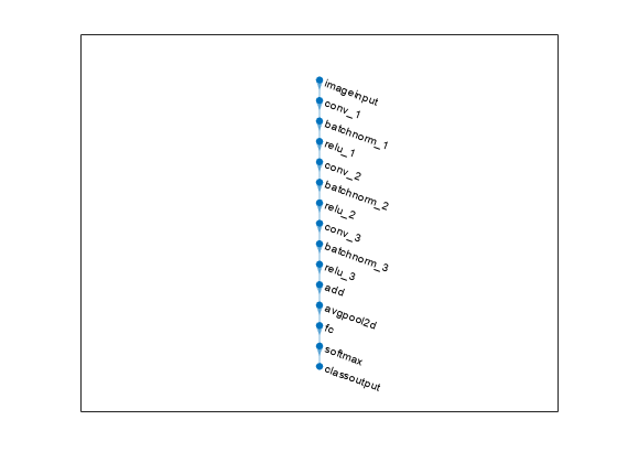
Create a layer graph from the layer array.layerGraphconnects all the layers inlayerssequentially. Plot the layer graph.

lgraph = layerGraph(layers); figure plot(lgraph)

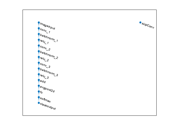
Create the 1-by-1 convolutional layer and add it to the layer graph. Specify the number of convolutional filters and the stride so that the activation size matches the activation size of the third ReLU layer. This arrangement enables the addition layer to add the outputs of the third ReLU layer and the 1-by-1 convolutional layer. To check that the layer is in the graph, plot the layer graph.

skipConv = convolution2dLayer(1,32,'Stride',2,'Name','skipConv'); lgraph = addLayers(lgraph,skipConv); figure plot(lgraph)

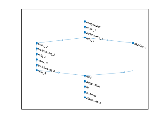
创建快捷方式连接from the'relu_1'layer to the'add'layer. Because you specified two as the number of inputs to the addition layer when you created it, the layer has two inputs named'in1'and'in2'. The third ReLU layer is already connected to the'in1'input. Connect the'relu_1'layer to the'skipConv'layer and the'skipConv'layer to the'in2'input of the'add'layer. The addition layer now sums the outputs of the third ReLU layer and the'skipConv'layer. To check that the layers are connected correctly, plot the layer graph.

lgraph = connectLayers(lgraph,'relu_1','skipConv'); lgraph = connectLayers(lgraph,'skipConv','add/in2'); figure plot(lgraph);

Load the training and validation data, which consists of 28-by-28 grayscale images of digits.

[XTrain,YTrain] = digitTrain4DArrayData; [XValidation,YValidation] = digitTest4DArrayData;

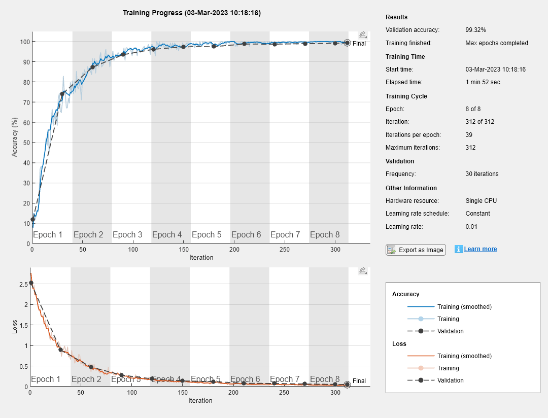
Specify training options and train the network.trainNetworkvalidates the network using the validation data everyValidationFrequencyiterations.

options = trainingOptions('sgdm',...“MaxEpochs”,8,...'Shuffle','every-epoch',...'ValidationData',{XValidation,YValidation},...'ValidationFrequency',30,...'Verbose',false,...“阴谋”,'training-progress'); net = trainNetwork(XTrain,YTrain,lgraph,options);

Display the properties of the trained network. The network is aDAGNetwork对象。

net

net = DAGNetwork with properties: Layers: [16x1 nnet.cnn.layer.Layer] Connections: [16x2 table] InputNames: {'imageinput'} OutputNames: {'classoutput'}

Classify the validation images and calculate the accuracy. The network is very accurate.

YPredicted = classify(net,XValidation); accuracy = mean(YPredicted == YValidation)

accuracy = 0.9934