Minimize Rastrigin's Function

Rastrigin's Function

This example shows how to find the minimum of Rastrigin's function, a function that is often used to test the genetic algorithm. The example presents two approaches for minimizing: using theOptimizeLive Editor task and working at the command line.

For two independent variables, Rastrigin's function is defined as

$R a s (x) = 20 + x_{1}^{2} + x_{2}^{2} - 10 (\cos 2 π x_{1} + \cos 2 π x_{2}) .$

Global Optimization Toolboxcontains therastriginsfcn.mfile, which computes the values of Rastrigin's function. The following figure shows a plot of Rastrigin's function.

As the plot shows, Rastrigin's function has many local minima—the “valleys” in the plot. However, the function has just one global minimum, which occurs at the point [0 0] in thex-yplane, as indicated by the vertical line in the plot, where the value of the function is 0. At any local minimum other than [0 0], the value of Rastrigin's function is greater than 0. The farther the local minimum is from the origin, the larger the value of the function is at that point.

Rastrigin's function is often used to test the genetic algorithm, because its many local minima make it difficult for standard, gradient-based methods to find the global minimum.

The following contour plot of Rastrigin's function shows the alternating maxima and minima.

Minimize Using theOptimizeLive Editor Task

This section explains how to find the minimum of Rastrigin's function using the genetic algorithm.

Note

Because the genetic algorithm uses random number generators, the algorithm returns different results each time you run it.

Create a new live script by clicking theNew Live Scriptbutton in theFilesection on theHometab.
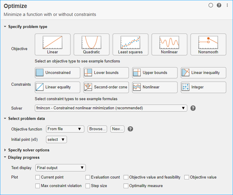
Insert anOptimizeLive Editor task. Click theInserttab and then, in theCodesection, selectTask > Optimize.
For use in entering problem data, insert a new section by clicking theSection Breakbutton on theInserttab. New sections appear above and below the task.
In the new section above the task, enter the following code to define the number of variables and objective function.
```
nvar = 2; fun = @rastriginsfcn;
```
To place these variables into the workspace, run the section by pressingCtrl+Enter.
In theSpecify problem typesection of the task, click theObjective > Nonlinear button.
SelectSolver > ga - Genetic algorithm.
In theSelect problem datasection of the task, selectObjective function > Function handleand then choosefun.
SelectNumber of variables > nvar.
In theDisplay progresssection of the task, select theBest fitnessplot.
To run the solver, click the options button⁝at the top right of the task window, and selectRun Section. The plot appears in a separate figure window and in the task output area. Note that your plot might be different from the one shown, becausegais a stochastic algorithm.

The points at the bottom of the plot denote the best fitness values, while the points above them denote the averages of the fitness values in each generation. The top of the plot displays the best and mean values, numerically, in the current generation.
To see the solution and fitness function value, look at the top of the task.
To view the values of these variables, enter the following code in the section below the task.
```
disp(solution) disp(objectiveValue)
```
Run the section by pressingCtrl+Enter.
```
disp(solution)
```
```
0.9785 0.9443
```
```
disp(objectiveValue)
```
```
2.5463
```
Your values can differ becausegais a stochastic algorithm.

The value shown is not very close to the actual minimum value of Rastrigin's function, which is0. The topicsSet Initial Range,Setting the Amount of Mutation, andSet Maximum Number of Generations and Stall Generationsdescribe ways to achieve a result that is closer to the actual minimum. Or, you can simply rerun the solver to try to obtain a better result.

Minimize at the Command Line

To find the minimum of Rastrigin's function at the command line, enter the following code.

rngdefault% For reproducibilityoptions = optimoptions('ga','PlotFcn','gaplotbestf'); [solution,objectiveValue] = ga(@rastriginsfcn,2,...[],[],[],[],[],[],[],options)

Best fitness and mean fitness decrease over nearly 60 generations

Optimization terminated: average change in the fitness value less than options.FunctionTolerance. solution = 0.9785 0.9443 objectiveValue = 2.5463

The points at the bottom of the plot denote the best fitness values, while the points above them denote the averages of the fitness values in each generation. The top of the plot displays the best and mean values, numerically, in the current generation.

Both theOptimizeLive Editor task and the command line allow you to formulate and solve problems, and they give identical results. The command line is more streamlined, but provides less help for choosing a solver, setting up the problem, and choosing options such as plot functions. You can also start a problem usingOptimize, and then generate code for command line use, as inSolve a Constrained Nonlinear Problem, Solver-Based.