在两极电机磁场

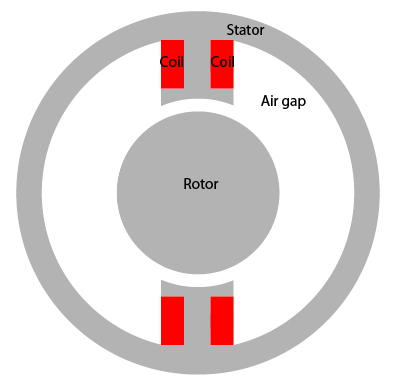
Find the static magnetic field induced by the stator windings in a two-pole electric motor. Assuming that the motor is long and the end effects are negligible, you can use a 2-D model. The geometry consists of three regions:

The magnetic permeability of air and of copper are both close to the magnetic permeability of a vacuum,μ=μ₀. The magnetic permeability of the stator and the rotor isμ= 5000μ₀. The current densityJis 0 everywhere except in the coil, where it is 10 A/m².

The geometry of the problem makes the magnetic vector potentialAsymmetric with respect to they-axis and antisymmetric with respect to thex-axis. Therefore, you can limit the domain tox≥ 0,y≥ 0, with the default boundary condition

on thex-axis and the boundary conditionA= 0 on they-axis. Because the field outside the motor is negligible, you can use the boundary conditionA= 0 on the exterior boundary.

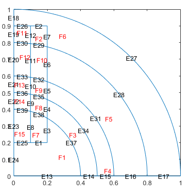
First, create the geometry in the PDE Modeler app. The geometry of this electric motor is a union of five circles and two rectangles. To draw the geometry, enter the following commands in the MATLAB^®Command Window:

pdecirc(0,0,1,“C1”) pdecirc(0,0,0.8,'C2') pdecirc(0,0,0.6,'C3') pdecirc(0,0,0.5,'C4') pdecirc(0,0,0.4,'C5') pderect([-0.2 0.2 0.2 0.9],'R1') pderect([-0.1 0.1 0.2 0.9],'R2') pderect([0 1 0 1],'SQ1')

Reduce the geometry to the first quadrant by intersecting it with a square. To do this, enter(C1+C2+C3+C4+C5+R1+R2)*SQ1in theSet formulafield.

From the PDE Modeler app, export the geometry description matrix, set formula, and name-space matrix to the MATLAB workspace by selectingExport Geometry Description, Set Formula, Labels...from theDrawmenu.

In the MATLAB Command Window, use thedecsgfunction to decompose the exported geometry into minimal regions. This command creates anAnalyticGeometryobjectd1. Plot the geometryd1.

[d1,bt1] = decsg(gd,sf,ns); pdegplot(d1,"EdgeLabels","on","FaceLabels","on")

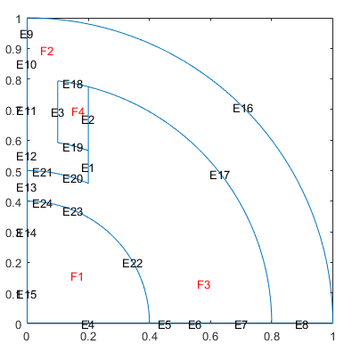
Remove unnecessary edges using thecsgdelfunction. Specify the edges to delete as a vector of edge IDs. Plot the resulting geometry.

[d2,bt2] = csgdel(d1,bt1,[1 3 8 25 7 2 12 26 30 33 4 9 34 10 31]); pdegplot(d2,"EdgeLabels","on","FaceLabels","on")

Create an electromagnetic model for magnetostatic analysis.

emagmodel = createpde("electromagnetic","magnetostatic");

Include the geometry in the model.

geometryFromEdges(emagmodel,d2);

Specify the vacuum permeability value in the SI system of units.

emagmodel.VacuumPermeability = 1.2566370614E-6;

Specify the relative permeability of the air gap and copper coil, which correspond to the faces 3 and 4 of the geometry.

electromagneticProperties(emagmodel,"RelativePermeability",1,..."Face",[3 4]);

Specify the relative permeability of the stator and the rotor, which correspond to the faces 1 and 2 of the geometry.

electromagneticProperties(emagmodel,"RelativePermeability",5000,..."Face",[1 2]);

Specify the current density in the coil.

electromagneticSource(emagmodel,"CurrentDensity",10,"Face",4);

Apply the zero magnetic potential condition to all boundaries, except the edges along thex-axis. The edges along thex-axis retain the default boundary condition.

electromagneticBC(emagmodel,"MagneticPotential",0,..."Edge",[16 9 10 11 12 13 14 15]);

Generate the mesh.

generateMesh(emagmodel);

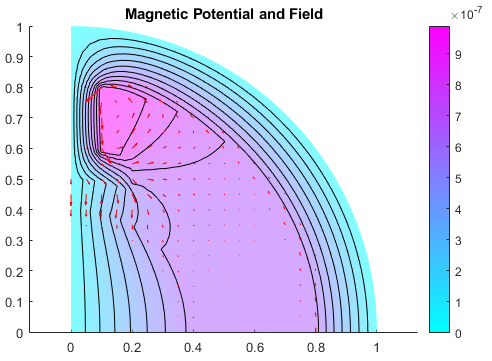
Solve the model and plot the magnetic potential. Use theContourparameter to display equipotential lines.

R = solve(emagmodel); figure pdeplot(emagmodel,“XYData”,R.MagneticPotential,"Contour","on") title"MagneticPotential"

Add the magnetic field data to the plot. Use theFaceAlphaparameter to make the quiver plot for magnetic field more visible.

figure pdeplot(emagmodel,“XYData”,R.MagneticPotential,..."FlowData",[R.MagneticField.Hx,...R.MagneticField.Hy],..."Contour","on",..."FaceAlpha",0.5) title"MagneticPotentialandField"