使用计量经济学建模器应用检测拱门效应
这些例子展示了如何评估时ther a series has volatility clustering by using theEconometric Modeler应用程序。方法包括检查平方残留物的相关图和对重要拱形滞后的测试。数据集存储在data_equitydx。mat, contains a series of daily NASDAQ closing prices from 1990 through 2001.
Inspect Correlograms of Squared Residuals for ARCH Effects
此示例显示了如何通过绘制一系列平方残差的自相关函数(ACF)和部分自相关函数(ACF)和部分自相关函数(ACF)和部分自相关函数(PACF)来视觉确定一个串联是否具有显着的弓形效应。
At the command line, load thedata_equitydx。matdata set.
loaddata_equitydx
数据集包含纳斯达克股票和纽约证券交易所收盘价的表,以及其他变量。有关数据集的更多详细信息,请输入描述at the command line.
Convert the tableDataTableto a timetable (for details, seePrepare Time Series Data for Econometric Modeler App)。
dates = dateTime(日期,“转换”,'datenum',。。。'Format','ddmmmyyyy');% Convert dates to datetimesdatatable.properties.rownames = {};%透明行名称dataTable = table2timetable(数据表,“行时”,dates);%将表转换为时间表
在命令行,打开Econometric Modeler应用程序。
计量经济学
Alternatively, open the app from the apps gallery (seeEconometric Modeler)。
ImportDataTable进入应用程序:
On theEconometric Modeler标签,在Importsection, click
 。
。在里面Import Datadialog box, in theImport?列,选择的复选框
DataTablevariable.ClickImport。
The variables appear in the时间序列窗格和所有系列的时间序列图出现在时间序列图(纳斯达克)figure window.
Convert the daily close NASDAQ index series to a percentage return series by taking the log of the series, then taking the first difference of the logged series:
在里面时间序列pane, select
NASDAQ。On theEconometric Modeler标签,在变换section, click日志。
With
Nasdaqlogselected, in the变换section, clickDifference。在里面时间序列pane, rename the
NasdaqlogDiff通过单击两次以选择其名称并输入的变量NASDAQReturns。
纳斯达克返回的时间序列图出现在时间序列Plot(NASDAQReturns)figure window.

The returns appear to fluctuate around a constant level, but exhibit volatility clustering. Large changes in the returns tend to cluster together, and small changes tend to cluster together. That is, the series exhibits conditional heteroscedasticity.
Compute squared residuals:
出口
NASDAQReturns到Matlab®工作区:在里面时间序列窗格,右键单击
NASDAQReturns。在里面context menu, select出口。
NASDAQReturns出现在MATLAB工作区中。At the command line:
For numerical stability, scale the returns by a factor of 100.
通过从缩放返回系列中删除平均值来创建残差系列。因为您花了纳斯达克价格的第一个区别来创建收益,所以退货的第一个要素丢失了。因此,要估计该系列的样本平均值,请致电
mean(NASDAQReturns,'omitnan')。Square the residuals.
Add the squared residuals as a new variable to the
DataTable时间表。
nasdaqreturns = 100*nasdaqreturns;nasdaqresiduals = nasdaqreturns-平均'omitnan');nasdaqresiduals2 = nasdaqresiduals。^2;datatable.nasdaqresiduals2 = nasdaqresiduals2;
In Econometric Modeler, importDataTable:
On theEconometric Modeler标签,在Importsection, click
。在里面Econometric Modeler对话框,单击好的to clear all variables and documents in the app.
在里面Import Datadialog box, in theImport?column, select the check box for
DataTable。ClickImport。
绘制ACF和PACF:
在里面时间序列pane, select the
nasdaqresiduals2time series.点击Plots标签,然后单击ACF。
点击Plots标签,然后单击PACF。
Close the时间序列图(纳斯达克)figure window. Then, position theACF(Nasdaqresiduals2)figure window above thePACF(NASDAQResiduals2)figure window.
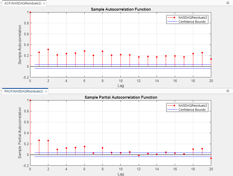
The sample ACF and PACF show significant autocorrelation in the squared residuals. This result indicates that volatility clustering is present.
Conduct Ljung-Box Q-Test on Squared Residuals
This example shows how to test squared residuals for significant ARCH effects using the Ljung-Box Q-test.
At the command line:
加载
data_equitydx。matdata set.将纳斯达克价格转换为回报。为了维持正确的时间基础,请用
NaNvalue.Scale the NASDAQ returns.
Compute residuals by removing the mean from the scaled returns.
Square the residuals.
Add the vector of squared residuals as a variable to
DataTable。Convert
DataTablefrom a table to a timetable.
有关步骤的更多详细信息,请参阅Inspect Correlograms of Squared Residuals for ARCH Effects。
loaddata_equitydxnasdaqreturns = 100*price2ret(datatable.nasdaq);nasdaqreturns = [nan;Nasdaqreturns];nasdaqresiduals2= (NASDAQReturns - mean(NASDAQReturns,'omitnan')。^2;datatable.nasdaqresiduals2 = nasdaqresiduals2;dates = dateTime(日期,“转换”,'datenum');datatable.properties.rownames = {};dataTable = table2timetable(数据表,“行时”,dates);
在命令行,打开Econometric Modeler应用程序。
计量经济学
Alternatively, open the app from the apps gallery (seeEconometric Modeler)。
ImportDataTable进入应用程序:
On theEconometric Modeler标签,在Importsection, click
。在里面Import Datadialog box, in theImport?列,选择的复选框
DataTablevariable.ClickImport。
The variables appear in the时间序列窗格和所有系列的时间序列图出现在时间序列图(纳斯达克)figure window.
Test the null hypothesis that the firstm= 5 autocorrelation lags of the squared residuals are jointly zero by using the Ljung-Box Q-test. Then, test the null hypothesis that the firstm=平方残差的10个自相关滞后滞后。
在里面时间序列pane, select the
nasdaqresiduals2time series.On theEconometric Modeler标签,在Testssection, click新测试>ljung-box q检验。
On theLBQ标签,在Parameters部分,设置both the滞后数和DOFto
5。为了保持两个测试的显着性水平为0.05,设置Significance Levelto 0.025.在里面Testssection, click运行测试。
Repeat steps 3 and 4, but set both the滞后数和DOFto
10instead.
测试结果出现在结果table of theLBQ(Nasdaqresiduals2)document.
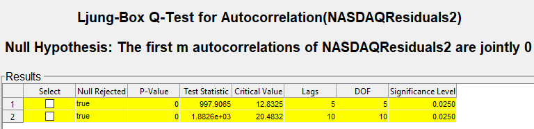
The null hypothesis is rejected for the two tests. Thep-value for each test is 0. The results show that not every autocorrelation up to lag 5 (or 10) is zero, indicating volatility clustering in the squared residuals.
进行Engle的拱门测试
This example shows how to test residuals for significant ARCH effects using the Engle's ARCH Test.
At the command line:
加载
data_equitydx。matdata set.将纳斯达克价格转换为回报。为了维持正确的时间基础,请用
NaNvalue.Scale the NASDAQ returns.
Compute residuals by removing the mean from the scaled returns.
Add the vector of residuals as a variable to
DataTable。Convert
DataTablefrom a table to a timetable.
有关步骤的更多详细信息,请参阅Inspect Correlograms of Squared Residuals for ARCH Effects。
loaddata_equitydxnasdaqreturns = 100*price2ret(datatable.nasdaq);nasdaqreturns = [nan;Nasdaqreturns];nasdaqresiduals = nasdaqreturns-平均'omitnan');DataTable.NASDAQResiduals = NASDAQResiduals; dates = datetime(dates,“转换”,'datenum');datatable.properties.rownames = {};dataTable = table2timetable(数据表,“行时”,dates);
在命令行,打开Econometric Modeler应用程序。
计量经济学
Alternatively, open the app from the apps gallery (seeEconometric Modeler)。
ImportDataTable进入应用程序:
On theEconometric Modeler标签,在Importsection, click
。在里面Import Datadialog box, in theImport?列,选择的复选框
DataTablevariable.ClickImport。
The variables appear in the时间序列pane, and a time series plot of the all the series appears in the时间序列图(纳斯达克)figure window.
Test the null hypothesis that the NASDAQ residuals series exhibits no ARCH effects by using Engle's ARCH test. Specify that the residuals series is an ARCH(2) model.
在里面时间序列pane, select the
NASDAQResidualstime series.On theEconometric Modeler标签,在Testssection, click新测试>恩格尔的拱门测试。
On theARCH标签,在Parameters部分,设置滞后数to
2。在里面Testssection, click运行测试。
测试结果出现在结果table of the拱门(纳斯达克利群岛)document.
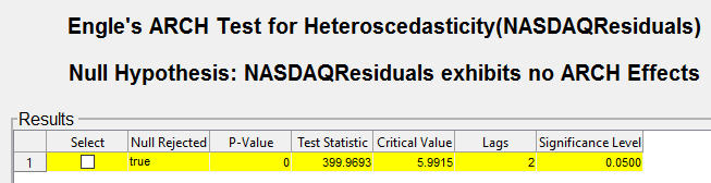
The null hypothesis is rejected in favor of the ARCH(2) alternative. The test result indicates significant volatility clustering in the residuals.