Antenna Diversity Analysis for 800 MHz MIMO

Open Live Script

This example analyzes a 2-antenna diversity scheme to understand the effect that position, orientation and frequency have on received signals. The analysis is performed under the assumptions that impedance matching is not achieved and mutual coupling is taken into account [1].

Frequency Band Parameters

Define the operating frequency, analysis bandwidth and calculate the wavelength in free space.

freq = 800e6; c = physconst('lightspeed'); lambda = c/freq; BW_frac = .1; fmin = freq - BW_frac*freq; fmax = freq + BW_frac*freq;

Create Two Identical Dipoles

Use the dipole antenna element from the Antenna Toolbox™ library and create 2 identical thin dipoles of length $λ / 2$ .

d1 = dipole('Length',lambda/2,'Width',lambda/200); d2 = dipole('Length',lambda/2,'Width',lambda/200);

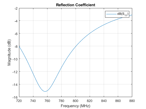
Plot Input Reflection Coefficient of Isolated Dipole

计算the input reflection coefficient of an isolated dipole and plot it to confirm the lack of impedance match at 800MHz.

Numfreq = 101; f = linspace(fmin,fmax,Numfreq); S = sparameters(d1,f); DipoleS11Fig = figure; rfplot(S,1,1) title('Reflection Coefficient')

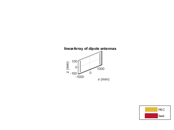
$Figure contains an axes object. The axes object with title Reflection Coefficient contains an object of type line. This object represents dB(S_{11}).$

Create Two-Element Array

Create the two-element antenna diversity system and position the 2 antennas apart by 5 $λ$ .

range = 5*lambda; l = linearArray; l.Element = [d1 d2]; l.ElementSpacing = range; show(l) view(-80,4)

Figure contains an axes object. The axes object with title linearArray of dipole antennas contains 6 objects of type patch, surface. These objects represent PEC, feed.

Power Transfer Function

计算并绘制功率传递函数(S21 in dB) for two antennas. To do so, calculate the scattering parameters for the system and plot S21 over the entire frequency range.

S = sparameters(l,f); ArrayS21Fig = figure; rfplot(S,2,1) title('Power Transfer Function')

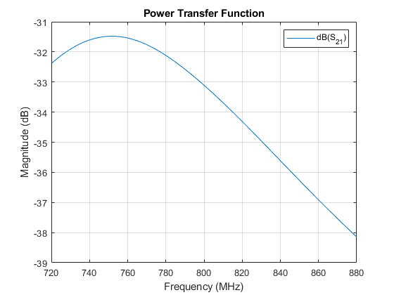
$Figure contains an axes object. The axes object with title Power Transfer Function contains an object of type line. This object represents dB(S_{21}).$

The response peak is clearly not at 800 MHz. In addition, note the loss in signal strength due to attenuation in free space.

Vary spatial orientation of dipole

Power transfer between the two antennas can now be investigated as a function of antenna orientation. A correlation coefficient is used in MIMO systems to quantify the system performance. Two approaches to calculate the correlation coefficient exist; using the far-field behavior and using the S-parameters. The field-based approach involves numerical integration. The calculation suggested in this example uses the function correlation available in the Antenna Toolbox™ and based on the S-parameters approach [1]. By rotating one antenna located on the positive x-axis, we change its polarization direction and find the correlation

numpos = 101; orientation = linspace(0,90,numpos); S21_TiltdB = nan(1,numel(orientation)); Corr_TiltdB = nan(1,numel(orientation)); fig1 = figure;fori = 1:numel(orientation) d2.Tilt = orientation(i); l.Element(2) = d2; S = sparameters(l,freq); Corr = correlation(l,freq,1,2); S21_TiltdB = 20*log10(abs(S.Parameters(2,1,1))); Corr_TiltdB(i) = 20*log10(Corr); figure(fig1); plot(orientation,S21_TiltdB,orientation,Corr_TiltdB,'LineWidth',2) gridonaxis([min(orientation) max(orientation) -65 -20]); xlabel('Tilt variation on 2nd dipole (deg.)') ylabel('Magnitude (dB)') title('Correlation, S_2_1 Variation with Polarization') drawnowendlegend('S_2_1','Correlation');

Figure contains an axes object. The axes object with title C o r r e l a t i o n , blank S indexOf 1 baseline blank blank V a r i a t i o n blank w i t h blank P o l a r i z a t i o n contains 102 objects of type line. These objects represent S_2_1, Correlation.

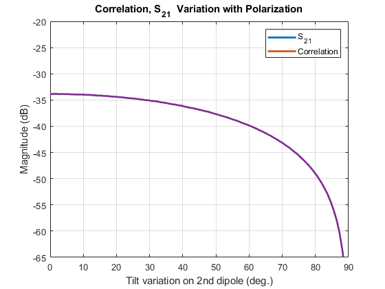
We observe that the power transfer function and the correlation function between the two antennas are identical as the antenna orientation changes for one of the dipoles.

Vary Spacing between Antennas

Restore both dipoles so that they are parallel to each other. Run a similar analysis by changing the spacing between the 2 elements.

d2.Tilt = 0; l.Element = [d1 d2]; Nrange = 201; Rmin = 0.001*lambda; Rmax = 2.5*lambda; range = linspace(Rmin,Rmax,Nrange); S21_RangedB = nan(1,Nrange); Corr_RangedB = nan(1,Nrange); fig2 = figure;fori = 1:Nrange l.ElementSpacing = range(i); S = sparameters(l,freq); Corr = correlation(l,freq,1,2); S21_RangedB(i)= 20*log10(abs(S.Parameters(2,1,1))); Corr_RangedB(i)= 20*log10(Corr); figure(fig2); plot(range./lambda,S21_RangedB,range./lambda,Corr_RangedB,'--','LineWidth',2) gridonaxis([min(range./lambda) max(range./lambda) -50 0]); xlabel('Distance of separation, d/\lambda') ylabel('Magnitude (dB)') title('Correlation, S_2_1 Variation with Range') drawnow holdoffendlegend('S_2_1','Correlation');

Figure contains an axes object. The axes object with title C o r r e l a t i o n , blank S indexOf 1 baseline blank V a r i a t i o n blank w i t h blank R a n g e contains 2 objects of type line. These objects represent S_2_1, Correlation.

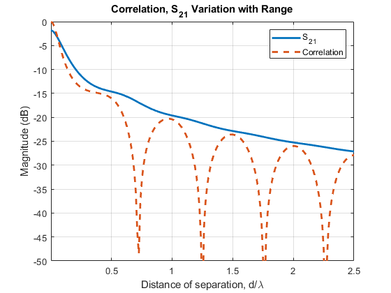
The 2 curves are clearly different in their behavior when the separation distance between two antennas increases. This plot reveals the correlation valleys that exist at specific separations such as approximately 0.75 $λ$ , 1.25 $λ$ , 1.75 $λ$ , and 2.25 $λ$ .

Check Correlation Frequency Response

Pick the separation to be 1.25 $λ$ , which is one of the correlation valleys. Analyze the correlation variation for 10% bandwidth centered at 800 MHz.

Rpick = 1.25*lambda; f = linspace(fmin,fmax,Numfreq); l.ElementSpacing = Rpick; Corr_PickdB = 20.*log10(correlation(l,f,1,2)); fig2 = figure; plot(f./1e9,Corr_TiltdB,'LineWidth',2) gridonaxis([min(f./1e9) max(f./1e9) -65 0]); xlabel('Frequency (GHz)') ylabel('Magnitude (dB)') title(“与频率相关变异”)

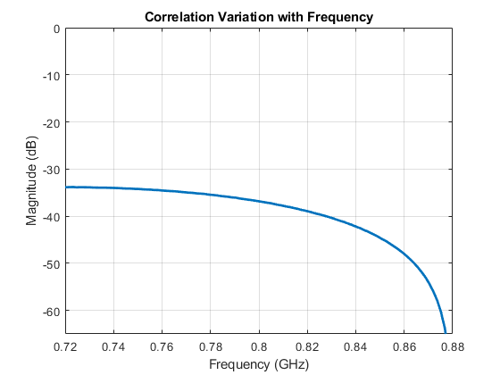
Figure contains an axes object. The axes object with title Correlation Variation with Frequency contains an object of type line.

The results of the analysis reveals that the two antennas have a correlation below 30 dB over the band specified.

Reference

[1] S. Blanch, J. Romeu, and I. Corbella, "Exact representation of antenna system diversity performance from input parameter description," Electron. Lett., vol. 39, pp. 705-707, May 2003. Online at:http://upcommons.upc.edu/e-prints/bitstream/2117/10272/4/ExactRepresentationAntenna.pdf