Gaussian Models
About Gaussian Models
The Gaussian model fits peaks, and is given by
whereais the amplitude,bis the centroid (location),cis related to the peak width,nis the number of peaks to fit, and 1 ≤n≤ 8.
Gaussian peaks are encountered in many areas of science and engineering. For example, Gaussian peaks can describe line emission spectra and chemical concentration assays.
Fit Gaussian Models Interactively
Open the Curve Fitter app by entering
curveFitterat the MATLAB®command line. Alternatively, on theAppstab, in theMath, Statistics and Optimizationgroup, clickCurve Fitter.In the Curve Fitter app, select curve data. On theCurve Fittertab, in theData部分中,点击Select Data. In theSelect Fitting Datadialog box, selectX DataandY Data, or justY Dataagainst an index.
Click the arrow in theFit Typesection to open the gallery, and clickGaussianin theRegression Modelsgroup.
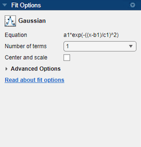
You can specify the following options in theFit Optionspane:
Specify the number of terms as a positive integer in the range [1 8]. Look in theResultspane to see the model terms, values of the coefficients, and goodness-of-fit statistics.
Optionally, in theAdvanced Optionssection, specify coefficient starting values and constraint bounds, or change algorithm settings. The app calculates optimized start points forGaussian合适,基于数据集。你可以override the start points and specify your own values in theFit Optionspane.
Gaussian fits have the width parameter
c1constrained with a lower bound of0. The default lower bounds for most library models are-Inf, which indicates that the coefficients are unconstrained.
For more information on the settings, seeSpecify Fit Options and Optimized Starting Points.
Fit Gaussian Models Using the fit Function
This example shows how to use thefitfunction to fit a Gaussian model to data.
The Gaussian library model is an input argument to thefitandfittypefunctions. Specify the model typegaussfollowed by the number of terms, e.g.,'gauss1'through'gauss8'.
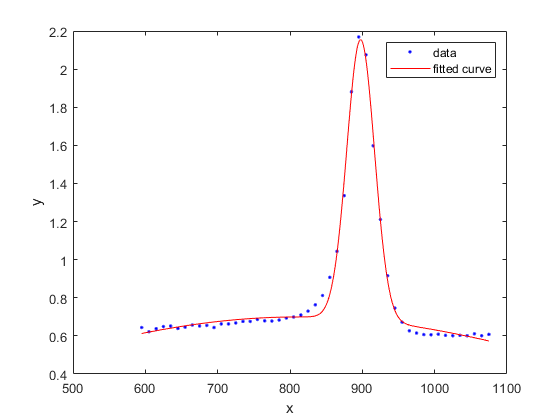
Fit a Two-Term Gaussian Model
Load some data and fit a two-term Gaussian model.
[x,y] = titanium; f = fit(x.',y.','gauss2')
f = General model Gauss2: f(x) = a1*exp(-((x-b1)/c1)^2) + a2*exp(-((x-b2)/c2)^2) Coefficients (with 95% confidence bounds): a1 = 1.47 (1.426, 1.515) b1 = 897.7 (897, 898.3) c1 = 27.08 (26.08, 28.08) a2 = 0.6994 (0.6821, 0.7167) b2 = 810.8 (790, 831.7) c2 = 592.9 (500.1, 685.7)
plot(f,x,y)
See Also
Apps
Functions
Related Topics
You can also select a web site from the following list:
Americas
- América Latina(Español)
- Canada(English)
- United States(English)
Europe
- Belgium(English)
- 丹麦(English)
- Deutschland(Deutsch)
- España(Español)
- Finland(English)
- France(Français)
- Ireland(English)
- Italia(Italiano)
- Luxembourg(English)
- Netherlands(English)
- Norway(English)
- Österreich(Deutsch)
- Portugal(English)
- Sweden(English)
- Switzerland
- United Kingdom(English)