Load Pretrained Network

Load the pretrained network from the supporting filedigitsNet.mat. This file contains a classification network that classifies handwritten digits.

loaddigitsNetlayers = net.Layers

layers = 15×1 Layer array with layers: 1 'imageinput' Image Input 28×28×1 images with 'zerocenter' normalization 2 'conv_1' Convolution 8 3×3×1 convolutions with stride [1 1] and padding 'same' 3 'batchnorm_1' Batch Normalization Batch normalization with 8 channels 4 'relu_1' ReLU ReLU 5 'maxpool_1' Max Pooling 2×2 max pooling with stride [2 2] and padding [0 0 0 0] 6 'conv_2' Convolution 16 3×3×8 convolutions with stride [1 1] and padding 'same' 7 'batchnorm_2' Batch Normalization Batch normalization with 16 channels 8 'relu_2' ReLU ReLU 9 'maxpool_2' Max Pooling 2×2 max pooling with stride [2 2] and padding [0 0 0 0] 10 'conv_3' Convolution 32 3×3×16 convolutions with stride [1 1] and padding 'same' 11 'batchnorm_3' Batch Normalization Batch normalization with 32 channels 12 'relu_3' ReLU ReLU 13 'fc' Fully Connected 10 fully connected layer 14 'softmax' Softmax softmax 15 'classoutput' Classification Output crossentropyex with '0' and 9 other classes

Load Data

The data set contains synthetic images of handwritten digits together with the corresponding angles (in degrees) by which each image is rotated.

Load the training and validation images as 4-D arrays usingdigitTrain4DArrayDataanddigitTest4DArrayData. The outputsYTrainandYValidationare the rotation angles in degrees. The training and validation data sets each contain 5000 images.

[XTrain,~,YTrain] = digitTrain4DArrayData; [XValidation,~,YValidation] = digitTest4DArrayData;

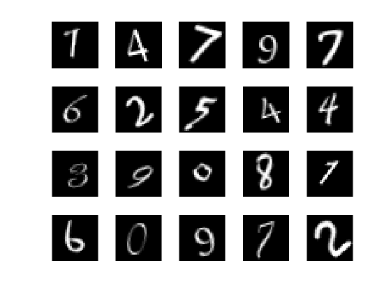
Display 20 random training images usingimshow.

numTrainImages = numel(YTrain); figure idx = randperm(numTrainImages,20);fori = 1:numel(idx) subplot(4,5,i) imshow(XTrain(:,:,:,idx(i)))end

Replace Final Layers

The convolutional layers of the network extract image features that the last learnable layer and the final classification layer use to classify the input image. These two layers,'fc'and'classoutput'indigitsNet, contain information on how to combine the features that the network extracts into class probabilities, a loss value, and predicted labels. To retrain a pretrained network for regression, replace these two layers with new layers adapted to the task.

Replace the final fully connected layer, the softmax layer, and the classification output layer with a fully connected layer of size 1 (the number of responses) and a regression layer.

numResponses = 1; layers = [ layers(1:12) fullyConnectedLayer(numResponses) regressionLayer];

Freeze Initial Layers

The network is now ready to be retrained on the new data. Optionally, you can "freeze" the weights of earlier layers in the network by setting the learning rates in those layers to zero. During training,trainNetworkdoes not update the parameters of the frozen layers. Because the gradients of the frozen layers do not need to be computed, freezing the weights of many initial layers can significantly speed up network training. If the new data set is small, then freezing earlier network layers can also prevent those layers from overfitting to the new data set.

Use the supporting functionfreezeWeightsto set the learning rates to zero in the first 12 layers.

layers(1:12) = freezeWeights(layers(1:12));

Train Network

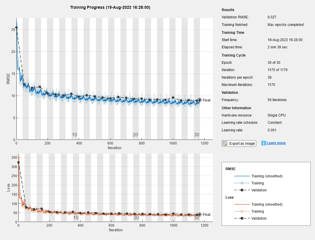
Create the network training options. Set the initial learn rate to 0.001. Monitor the network accuracy during training by specifying validation data. Turn on the training progress plot, and turn off the command window output.

options = trainingOptions('sgdm',...'InitialLearnRate',0.001,...'ValidationData',{XValidation,YValidation},...'Plots','training-progress',...'Verbose',false);

Create the network usingtrainNetwork. This command uses a compatible GPU if available. Using a GPU requires Parallel Computing Toolbox™ and a supported GPU device. For information on supported devices, seeGPU Support by Release(Parallel Computing Toolbox). Otherwise,trainNetworkuses the CPU.

net = trainNetwork(XTrain,YTrain,layers,options);

Test Network

Test the performance of the network by evaluating the accuracy on the validation data.

Usepredictto predict the angles of rotation of the validation images.

YPred = predict(net,XValidation);

Evaluate the performance of the model by calculating:

Calculate the prediction error between the predicted and actual angles of rotation.

predictionError = YValidation - YPred;

计算预测的数量在一个访问ptable error margin from the true angles. Set the threshold to be 10 degrees. Calculate the percentage of predictions within this threshold.

thr = 10; numCorrect = sum(abs(predictionError) < thr); numImagesValidation = numel(YValidation); accuracy = numCorrect/numImagesValidation

accuracy = 0.7532

Use the root-mean-square error (RMSE) to measure the differences between the predicted and actual angles of rotation.

rmse = sqrt(mean(predictionError.^2))

rmse =single9.0270

Correct Digit Rotations

You can use functions from Image Processing Toolbox to straighten the digits and display them together. Rotate 49 sample digits according to their predicted angles of rotation usingimrotate(Image Processing Toolbox).

idx = randperm(numImagesValidation,49);fori = 1:numel(idx) I = XValidation(:,:,:,idx(i)); Y = YPred(idx(i)); XValidationCorrected(:,:,:,i) = imrotate(I,Y,'bicubic','crop');end

Display the original digits with their corrected rotations. Usemontage(Image Processing Toolbox) to display the digits together in a single image.

figure subplot(1,2,1) montage(XValidation(:,:,:,idx)) title('Original') subplot(1,2,2) montage(XValidationCorrected) title('Corrected')