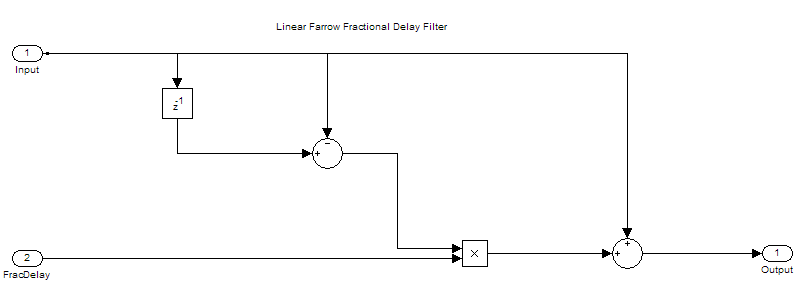
使用Farrow结构的分数延迟滤波器
此示例示出了如何设计所使用的Farrow结构实现的数字分数延迟滤波器。数字分数延迟(fracDelay)过滤器是有用的工具,以微调的信号的采样时刻。它们是,例如,通常在数字调制解调器的同步,其中延迟参数随时间变化的发现。这个例子说明了Farrow结构,用于实现随时间变化的FIR滤波器fracDelay一种流行的方法。
理想分数延迟滤波器
理想的分数延迟滤波器是线性相位全通滤波器。其脉冲响应是时间移位的离散正弦函数对应于一个非因果滤波器。由于脉冲响应是无限的,它不能被通过在时间上的有限移制成因果。因此,无变现,必须近似。
法罗结构
为了计算分数阶延迟滤波器的输出,我们需要估计现有离散时间样本之间的输入信号的值。可以使用特殊的插值滤波器来计算任意点处的新采样值。其中,基于多项式的滤波器特别有趣,因为一种特殊的结构——法罗结构——允许对系数进行简单的处理。特别是,Farrow结构的可调性使其非常适合实际的硬件实现。

最大平坦FIR近似(拉格朗日插值)
拉格朗日插值是一种时域方法,它导致了基于多项式的滤波器的特殊情况。输出信号近似为M次多项式。最简单的情况(M=1)对应于线性插值。让我们设计并分析一个线性分数延迟滤波器,它将单位延迟分成不同的分数:
Nx = 1024;Nf = 5;yw = 0 (Nx、Nf);transferFuncEstimator = dsp.TransferFunctionEstimator (...“SpectralAverages”25岁的'频率范围','片面');arrPlotPhaseDelay = dsp.ArrayPlot (“PlotType”,“行”,“YLimits”,[0 1.5],...'YLabel',的相位延迟,'SampleIncrement',1/512);arrPlotMag = dsp.ArrayPlot (“PlotType”,“行”,“YLimits”,-10年[1],...'YLabel',“(dB)级”,'SampleIncrement',1/512);fracDelay = dsp.VariableFractionalDelay;xw = randn (Nx、Nf);transferFuncEstimator(XW,YW);w = getFrequencyVector (transferFuncEstimator, 2 *π);w = repmat (w 1 Nf);抽搐,而toc < 2yw = fracDelay(xw,[0 0.2 0.4 0.6 0.8]);H = transferFuncEstimator (xw yw);arrPlotMag (20 * log10 (abs (H))) arrPlotPhaseDelay(角(H) / w)。结束释放(transferFuncEstimator)释放(arrPlotMag)释放(arrPlotPhaseDelay)释放(fracDelay)
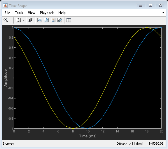
对于延迟的任何值,理想的过滤器应该同时具有平坦幅度响应和一个平坦的相位延迟的响应。近似只对最低频率是正确的。这意味着在实践中,信号需要过采样的线性分数延迟到正常工作。在这里,您申请两个不同的分数延迟正弦波和使用的时间范围覆盖原来的正弦波和两个延迟版本。0.2样品用1000Hz的采样速率的延迟,对应于0.2毫秒的延迟。
范围= dsp.TimeScope (“SampleRate”,1000,...“YLimits”[1],...“时间间隔”只有,...'TimeSpanOverrunAction','滚动');正弦= dsp.SineWave('频率',50岁,“SamplesPerFrame”Nx);抽搐,而toc < 2 x = sin ();y = fracDelay (x)。2。8]);%延迟0.2毫秒和0.8毫秒范围([x, y (: 1), y (:, 2)))结束释放(范围);发行版(fracDelay)

高阶Lagrange插值可以设计。让我们来比较的三次拉格朗日插值与线性之一:
farrowFracDelay = dsp.VariableFractionalDelay (...“InterpolationMethod”,“法罗”,“MaximumDelay”,1025);
Nf = 2;yw = 0 (Nx、Nf);xw = randn (Nx、Nf);H = transferFuncEstimator (xw yw);w = getFrequencyVector (transferFuncEstimator, 2 *π);w = repmat (w 1 Nf);抽搐,而toc < 2%,持续2秒,运行yw (: 1) = fracDelay (xw (: 1), 0.4);延迟0.4毫秒yw (:, 2) = farrowFracDelay (xw (:, 2), 1.4);%延迟1.4毫秒H = transferFuncEstimator (xw yw);arrPlotMag(20 *日志10(ABS(H)))arrPlotPhaseDelay(-unwrap(角(H))./ w)的结束释放(transferFuncEstimator)释放(arrPlotMag)释放(arrPlotPhaseDelay)释放(fracDelay)
Increasing the order of the polynomials slightly increases the useful bandwidth when Lagrange approximation is used, the length of the differentiating filters i.e. the number of pieces of the impulse response (number of rows of the 'Coefficients' property) is equal to the length of the polynomials (number of columns of the 'Coefficients' property). Other design methods can be used to overcome this limitation. Also notice how the phase delay of the third order filter is shifted from 0.4 to 1.4 samples at DC. Since the cubic lagrange interpolator is a 3rd order filter, the minimum delay it can achieve is 1. For this reason, the delay requested is 1.4 ms instead of 0.4 ms for this case.
正弦= dsp.SineWave('频率',50岁,“SamplesPerFrame”Nx);抽搐,而toc < 2 x = sin ();日元= fracDelay (x, 0.4);y2 = farrowFracDelay (x, 1.4);范围([x, y1, y2])结束释放(范围);发行版(fracDelay)

时变分数延迟
与直接形式的FIR相比,Farrow结构的优点在于它的可调性。在许多实际应用中,延迟是时变的。对于每一个新的延迟,我们将需要一组新的系数在直接形式的实现,但与Farrow实现,多项式系数保持不变。
抽搐,而toc < 5 x = sin ();如果toc < 1延迟= 1;elseiftoc < 2延迟= 1.2;elseiftoc < 3延迟= 1.4;elseiftoc < 4延迟= 1.6;其他的延迟= 1.8;结束y = farrowFracDelay (x,延迟);范围((x, y))结束释放(范围);发行版(fracDelay)
您还可以选择从下面的列表中的网站: