bigimageshow
Display 2-DblockedImageobject
Description
Abigimageshowobject displays data from ablockedImageobject. Thebigimageshow我对象逐步加载mage data based on image extents and screen resolution.
Creation
Syntax
Description
bigimageshow(displays the 2-D blocked imagebim)bim.
For categorical data,bigimageshowsets the axis colormap toparula. For numeric data,grayis the default colormap.
b = bigimageshow(___)returns thebigimageshowobjectb. Usebto modify the display settings after you display the blocked image.
b= bigimageshow(___,Name,Value)
For example,bigimageshow(bim,'GridVisible','on','GridLineStyle',':')displays the blocked image,bim, and overlays dotted grid lines.
Input Arguments
Properties
Parent—Parent axes ofbigimageshowobject
gca(default) |axesobject
Parent axes of thebigimageshowobject, specified as anaxesobject. If you do not specify a parent,bigimageshowuses the handle to the current figure,gca. If a figure does not exist,bigimageshowcreates a new figure.
CData—2-DblockedImageobject to display
blockedImageobject
2-DblockedImageobject to display, specified as ablockedImageobject.
CDataMapping—Color data mapping method
'direct'(default) |'scaled'
Color data mapping method, specified as'direct'or'scaled'. Use this property to control the mapping of color data values inCDatainto the colormap.CDatamust be a vector or a matrix defining indexed colors. This property has no effect ifCDatais a 3-D array defining RGB colors.
The methods have these effects:
'direct'— Interpret the values as indices into the current colormap. Values with a decimal portion are fixed to the nearest lower integer.If the values are of type
doubleorsingle, values of1or less map to the first color in the colormap. Values equal to or greater than the length of the colormap map to the last color in the colormap.If the values are of type
uint8,uint16,uint32,uint64,int8,int16,int32,或int64, values of0or less map to the first color in the colormap. Values equal to or greater than the length of the colormap map to the last color in the colormap (or up to the range limits of the type).If the values are of type
logical, values of0map to the first color in the colormap and values of1map to the second color in the colormap.
'scaled'— Scale the values to range between the minimum and maximum color limits. TheCLimproperty of the axes contains the color limits.
AlphaData—Transparency data
1(default) |numeric scalar|blockedImageobject
Transparency data, specified in one of these forms:
Numeric scalar — Use a consistent transparency across the entire image.
2-D
blockedImageobject — Transparency data must have the same rows and columns extent as theCData2-DblockedImageobject. The blocked image can have multiple resolution levels, in which case,bigimageshowselects the level closest to the currentResolutionLevelfor display.
TheAlphaDataMappingproperty controls how MATLAB®interprets the alpha data transparency values.
Example:0.5
Data Types:single|double|int8|int16|int32|int64|uint8|uint16|uint32|uint64|logical
AlphaDataMapping—Interpretation ofAlphaDatavalues
'none'(default) |'scaled'|'direct'
Interpretation ofAlphaDatavalues, specified as one of these values:
'none'— Interpret the values as transparency values. A value of 1 or greater is completely opaque, a value of 0 or less is completely transparent, and a value between 0 and 1 is semitransparent.'scaled'— Map the values into the figure’s alphamap. The minimum and maximum alpha limits of the axes determine the alpha data values that map to the first and last elements in the alphamap, respectively. For example, if the alpha limits are[3 5], alpha data values less than or equal to3map to the first element in the alphamap. Alpha data values greater than or equal to5map to the last element in the alphamap. TheALimproperty of the axes contains the alpha limits. TheAlphamapproperty of the figure contains the alphamap.'direct'— Interpret the values as indices into the figure’s alphamap. Values with a decimal portion are fixed to the nearest lower integer:If the values are of type
doubleorsingle, values of 1 or less map to the first element in the alphamap. Values equal to or greater than the length of the alphamap map to the last element in the alphamap.If the values are of type integer, then values of 0 or less map to the first element in the alphamap. Values equal to or greater than the length of the alphamap map to the last element in the alphamap (or up to the range limits of the type). The integer types are
uint8,uint16,uint32,uint64,int8,int16,int32, andint64.If the values are of type
logical, values of0map to the first element in the alphamap and values of1map to the second element in the alphamap.
ResolutionLevel—Resolution level
正整数|'fine'|'coarse'
Resolution level of the 2-DblockedImageobject to display, specified as a positive integer that identifies a resolution level of the 2-DblockedImageobject in the CData property. Resolution level can also be specified as'fine'or'coarse'corresponding to these two limits. The default value is computed based on available screen space and resolution.
ResolutionLevelMode—Selection mode for resolution level
'auto'(default) |'manual'
Selection mode for resolution level, specified as one of these values:
'auto'— Automatically select resolution level based on parent axes and available screen size.'manual'— Manually specify resolution level by setting theResolutionLevelproperty.
GridVisible—Grid visibility
'off'(default) |'on'
Grid visibility, specified as'off'or'on'.bigimageshowspaces the grid in world units to include as many pixels as specified byCData.BlockSizeat the currentGridResolutionLevel.
GridLevel—Resolution level of blocked image at which to show grid
正整数|'fine'|'coarse'
Resolution level of blocked image at which to show grid, specified as one of these values:
正整数— Display the grid specified as a numeric scalar that identifies a resolution level of the 2-D
blockedImageobject in CData property. Value is between 1 and the value of theNumLevelsproperty of the blocked image in thebigimageshowCDataproperty.'fine'— Display the grid at the finest resolution level.'coarse'— Display the grid at the coarsest resolution level.
By default,GridLevelhas the same value asResolutionLevelproperty.
GridLevelMode—Selection mode for grid level
'auto'(default) |'manual'
Selection mode for grid level, specified as one of these values:
'auto'— Select the grid resolution level to match the image data resolution levelResolutionLevel.'manual'— Manually specify the grid resolution level by setting theGridLevelproperty.
GridColor—网格线color
'blue'(default) |RGB triplet|hexadecimal color code|color name|short color name
网格线color, specified as an RGB triplet, a hexadecimal color code, a color name, or a short color name. To display the grid lines, set theGridVisibleproperty to'on'.
For a custom color, specify an RGB triplet or a hexadecimal color code.
An RGB triplet is a three-element row vector whose elements specify the intensities of the red, green, and blue components of the color. The intensities must be in the range
[0,1]; for example,[0.4 0.6 0.7].A hexadecimal color code is a character vector or a string scalar that starts with a hash symbol (
#) followed by three or six hexadecimal digits, which can range from0toF. The values are not case sensitive. Thus, the color codes'#FF8800','#ff8800','#F80', and'#f80'are equivalent.
Alternatively, you can specify some common colors by name. This table lists the named color options, the equivalent RGB triplets, and hexadecimal color codes.
| Color Name | Short Name | RGB Triplet | Hexadecimal Color Code | Appearance |
|---|---|---|---|---|
'red' |
'r' |
[1 0 0] |
'#FF0000' |
|
'green' |
'g' |
[0 1 0] |
'#00FF00' |
|
'blue' |
'b' |
[0 0 1] |
'#0000FF' |
|
'cyan' |
'c' |
[0 1 1] |
'#00FFFF' |
|
'magenta' |
'm' |
[1 0 1] |
'#FF00FF' |
|
'yellow' |
'y' |
[1 1 0] |
'#FFFF00' |
|
'black' |
'k' |
[0 0 0] |
'#000000' |
|
'white' |
'w' |
[1 1 1] |
'#FFFFFF' |
|
Here are the RGB triplets and hexadecimal color codes for the default colors MATLAB uses in many types of plots.
| RGB Triplet | Hexadecimal Color Code | Appearance |
|---|---|---|
[0 0.4470 0.7410] |
'#0072BD' |
|
[0.8500 0.3250 0.0980] |
'#D95319' |
|
[0.9290 0.6940 0.1250] |
'#EDB120' |
|
[0.4940 0.1840 0.5560] |
'#7E2F8E' |
|
[0.4660 0.6740 0.1880] |
'#77AC30' |
|
[0.3010 0.7450 0.9330] |
'#4DBEEE' |
|
[0.6350 0.0780 0.1840] |
'#A2142F' |
|
Example:b.GridColor = [1 0 0]
Example:b.GridColor = 'r'
Example:b.GridColor = 'red'
Example:b.GridColor = '#FF0000'
GridAlpha—网格线transparency
0.8(default) |value in the range [0,1]
网格线transparency, specified as a value in the range [0, 1]. A value of1means completely opaque and a value of0means completely transparent. To display the grid lines, set theGridVisibleproperty to'on'.
GridLineWidth—网格线width
1(default) |positive numeric value
网格线width, specified as a positive numeric value, measured in points. To display the grid lines, set theGridVisibleproperty to'on'.
GridLineStyle—网格线style
“- - -”(default) |'--'|':'|'-.'
网格线style, specified as one of the line styles in this table.
| Line Style | Description | Resulting Line |
|---|---|---|
“- - -” |
Solid line |
|
'--' |
Dashed line |
|
':' |
虚线 |
|
'-.' |
Dash-dot line |
|
To display the grid lines, set theGridVisibleproperty to'on'.
Interpolation—插值法
'linear'(default) |'nearest'
插值法used to resample pixels, specified as'linear'for bilinear interpolation, or'nearest'for nearest neighbor interpolation.
For categorical data,bigimageshowsupports only nearest neighbor interpolation. For logical data, the default value is'nearest'.
On Windows systems with a software version of OpenGL, the only supported interpolation option is'nearest'.
可见—Control image visibility
'on'(default) |'off'
Control image visibility, specified as one of these values:
'on'— Display thebigimageshowobject.'off'— Hide the object without deleting it. You still can access the properties of an invisible object.
Object Functions
showmask |
Show mask overlay at specified inclusion threshold |
hidemask |
Hide mask overlay inbigimageshowobject |
showlabels |
Display label overlay onbigimageshowobject |
hidelabels |
Hide label overlay onbigimageshowobject |
Examples
Visualize 2-D Blocked Image at Different Resolution Levels
This example uses a modified version of a training image of a lymph node containing tumor tissue (tumor_091.tif) from the CAMELYON16 data set. The modified image has three coarse resolution levels and has been adjusted to enforce a consistent aspect ratio and to register features at each level.
Create a blocked image from the sample image.
bim = blockedImage('tumor_091R.tif');
Display the blocked image.
h = bigimageshow(bim);

Zoom in on a region in the image.
xlim([2100, 2600]) ylim([1800 2300])

To view the image at the three resolution levels, specify a new value for theResolutionLevelproperty. As you view each resolution level, note that the axis limits remain the same, butbigimageshowensures that the images from other levels are correctly sized. When you setResolutionLevel,ResolutionLevelModevalue changes to'manual'automatically.
h.ResolutionLevel = 3; pause(1); h.ResolutionLevel = 2; pause(1); h.ResolutionLevel = 1; pause(1);

Visualize Blocked Image with Grid Lines Indicating Blocks
Create a blocked image from the sample imagetumor_091R.tif. This sample image is a training image of a lymph node containing tumor tissue from the CAMELYON16 data set. The image has been modified to have three coarse resolution levels, and has been adjusted to enforce a consistent aspect ratio and to register features at each level.
bim = blockedImage('tumor_091R.tif','BlockSize', [128 128]);
Display the blocked image withbigimageshow. Specify that you want the grid to be visible at the finest resolution level (level 1). Also specify the color, width, and transparency of the grid lines.
h = bigimageshow(bim,...'GridVisible','on','GridLevel',1,...'GridLineWidth', 2,'GridColor','k','GridAlpha',0.3);

Validate Mask using Alpha Layer
Create a blocked image from the sample imagetumor_091R.tif. This sample image is a training image of a lymph node containing tumor tissue from the CAMELYON16 data set. The image has been modified to have three coarse resolution levels, and has been adjusted to enforce a consistent aspect ratio and to register features at each level.
bim = blockedImage('tumor_091R.tif');
Create a coarse mask using theblockedImageapplyobject function.
bmask = apply(bim, @(bs)im2gray(bs.Data)<120,"Level", 3);
Overlay the mask as an alpha layer.
ha1 = subplot(1,2,1); h = bigimageshow(bim); h.AlphaData = bmask; h.AlphaDataMapping ='direct'; alphamap([0.4 1]) h.Parent.Color ='r';

Independently visualize the mask.
ha2 = subplot(1,2,2); bigimageshow(bmask); linkaxes([ha1, ha2]);%

Improve Mask Creation Using InclusionThreshold and BlockSize
Create a blocked image from the sample imagetumor_091R.tif. This sample image is a training image of a lymph node containing tumor tissue from the CAMELYON16 data set. The image has been modified to have three coarse resolution levels, and has been adjusted to enforce a consistent aspect ratio and to register features at each level.
bim = blockedImage('tumor_091R.tif');
Create a mask using the coarsest resolution level of the blocked image.
bmask = apply(bim, @(im)im2gray(im.Data)<120,"Level", 3);
Display the blocked image with the mask.
h = bigimageshow(bim); showmask(h, bmask);

Experiment with different inclusion thresholds to get a better fit of the mask over the stained area. By default, the inclusion threshold is 0.5.
showmask(h, bmask,'InclusionThreshold', 0.2); showmask(h, bmask,'InclusionThreshold', 0); showmask(h, bmask,'InclusionThreshold', 0.06);

Experiment with different different block sizes, in conjunction with different inclusion thresholds, to get a better fit of the mask over the stained area. By default, the block size for the coarsest resolution level is 625-by-670.
showmask(h, bmask,'InclusionThreshold', 0.06,'BlockSize', [256 256]); showmask(h, bmask,'InclusionThreshold', 0.14,'BlockSize', [256 256]);

When you are satisfied with the mask, use it to segment the lymph node.
bls = selectBlockLocations(bim,'BlockSize', [256 256],...'Mask', bmask,'InclusionThreshold', 0.14); bregion = apply(bim, @(bs)bs.Data,'BlockLocationSet', bls); figure bigimageshow(bregion);%


Display Blocked Image with Label Overlay
Create a blocked image from the sample imagetumor_091R.tif. This sample image is a training image of a lymph node containing tumor tissue from the CAMELYON16 data set. The image has been modified to have three coarse resolution levels, and has been adjusted to enforce a consistent aspect ratio and to register features at each level.
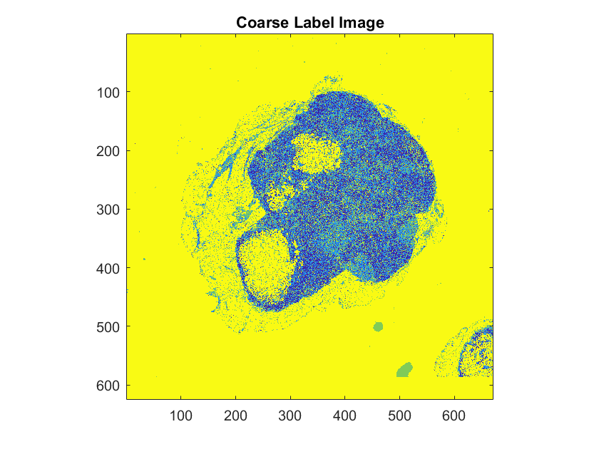
bim = blockedImage("tumor_091R.tif");
Create a label image at a coarse resolution level.
First get a single-resolution image. By default,gathergets data from the coarsest resolution level.
cim = gather(bim);
将图像转换为灰度。使用multithreshto calculate three threshold values to convert the image into a four-level image.
cgim = im2gray(cim); numClasses = 4; thresh = multithresh(cgim,numClasses-1);
Segment the image into four regions usingimquantize, specifying the threshold levels returned bymultithresh.
labels = imquantize(cgim,thresh); imagesc(labels) axissquaretitle("Coarse Label Image")
Convert thelabelsimage back to ablockedImageobject, using the same spatial referencing as the original image at the coarsest resolution level.
blabels = blockedImage(labels,WorldStart=bim.WorldStart(3,1:2),...WorldEnd=bim.WorldEnd(3,1:2));
Display the original blocked image.
figure hB = bigimageshow(bim);

Overlay thelabelsimage on the original blocked image.
showlabels(hB,blabels)

References
[1]
[2]
Version History
See Also
You can also select a web site from the following list:
Americas
- América Latina(Español)
- Canada(English)
- United States(English)
Europe
- Belgium(English)
- Denmark(English)
- Deutschland(Deutsch)
- España(Español)
- Finland(English)
- France(Français)
- Ireland(English)
- Italia(Italiano)
- Luxembourg(English)
- Netherlands(English)
- Norway(English)
- Österreich(Deutsch)
- Portugal(English)
- Sweden(English)
- Switzerland
- United Kingdom(English)