Differential Equations

Open Live Script

This example shows how to use MATLAB® to formulate and solve several different types of differential equations. MATLAB offers several numerical algorithms to solve a wide variety of differential equations:

Initial value problems
Boundary value problems
延迟微分方程
Partial differential equations

初始值问题

Vanderpoldemois a function that defines the van der Pol equation

$\frac{d^{2} y}{d t^{2}} - μ （（ 1 - y^{2} ） \frac{d y}{d t} + y = 0 。$

类型Vanderpoldemo

function dydt = vanderpoldemo(t,y,Mu) %VANDERPOLDEMO Defines the van der Pol equation for ODEDEMO. % Copyright 1984-2014 The MathWorks, Inc. dydt = [y(2); Mu*(1-y(1)^2)*y(2)-y(1)];

该方程式写为两个一阶普通微分方程（ODE）的系统。评估这些方程的参数值 $μ$ 。为了faster integration, you should choose an appropriate solver based on the value of $μ$ 。

为了 $μ = 1$ ，任何MATLAB ODE求解器都可以有效地求解Van der pol方程。这ode45solver is one such example. The equation is solved in the domain $[[0 ，，，， 20 这是给予的$ 有初始条件 $y （（ 0 ） = 2$ and $\frac{dy}{DT} |_{t = 0} = 0$ 。

tspan = [0 20]; y0 = [2; 0]; Mu = 1; ode = @(t,y) vanderpoldemo(t,y,Mu); [t,y] = ode45(ode, tspan, y0);％情节解决方案plot(t,y(:,1)) xlabel('t'）ylabel（'solution y'）title('van der pol方程，\ mu = 1'）

图包含一个轴对象。带有标题v a n空白的轴对象空白p o l空白e q u a t i o n，空白穆布空白=空白1包含一个类型行的对象。

为了larger magnitudes of $μ$ ，，，，the problem becomes僵硬的。该标签是针对抵制使用普通技术进行评估的问题的问题。相反，需要特殊的数值方法进行快速集成。这ODE15S，，，，ODE23S，，，，ode23t，，，，andode23tb功能可以有效地解决严重的问题。

此解决方案的解决方案 $μ = 1000$ 你sesODE15S具有相同的初始条件。您需要大幅度地延长时间到 $[[0 ，，，， 3000 这是给予的$ 能够看到解决方案的周期性运动。

tspan = [0, 3000]; y0 = [2; 0]; Mu = 1000; ode = @(t,y) vanderpoldemo(t,y,Mu); [t,y] = ode15s(ode, tspan, y0); plot(t,y(:,1)) title('van der pol方程，\ mu = 1000'）轴（[0 3000 -3 3]）Xlabel（'t'）ylabel（'solution y'）

图包含一个轴对象。这axes object with title v a n blank d e r blank P o l blank E q u a t i o n , blank mu blank = blank 1 0 0 0 contains an object of type line.

边界价值问题

bvp4candbvp5csolve boundary value problems for ordinary differential equations.

示例函数twoode具有一个微分方程为两个一阶ODE的系统。微分方程是

$\frac{d^{2} y}{d t^{2}} + | y | = 0 。$

类型twoode

function dydx = twoode(x,y) %TWOODE Evaluate the differential equations for TWOBVP. % % See also TWOBC, TWOBVP. % Lawrence F. Shampine and Jacek Kierzenka % Copyright 1984-2014 The MathWorks, Inc. dydx = [ y(2); -abs(y(1)) ];

这functiontwobc有问题的边界条件： $y （（ 0 ） = 0$ and $y （（ 4 ） = - 2$ 。

类型twobc

函数res = twOBC（YA，YB）％TWOBC评估在TWOBVP边界条件下的残差。％％参见Twoode，TwoBvp。％Lawrence F. Shampine和Jacek Kierzenka％版权1984-2014 The Mathworks，Inc。res = [YA（1）;YB（1） + 2];

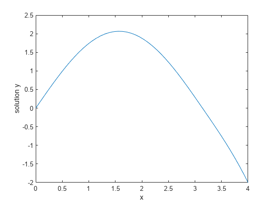
在打电话之前bvp4c，，，，you have to provide a guess for the solution you want represented at a mesh. The solver then adapts the mesh as it refines the solution.

这bvpinitfunction assembles the initial guess in a form you can pass to the solverbvp4c。为了a mesh of[[01234这是给予的和不断的猜测 $y （（ X ） = 1$ and $是的（（ X ） = 0$ ，打电话bvpinit是：

solinit = bvpinit（[0 1 2 3 4]，[1; 0]）;

With this initial guess, you can solve the problem withbvp4c。评估返回的解决方案bvp4c在某些时候使用deval，然后绘制结果值。

sol = bvp4c(@twoode, @twobc, solinit); xint = linspace(0, 4, 50); yint = deval(sol, xint); plot(xint, yint(1,:)); xlabel('X'）ylabel（'solution y'）holdon

图包含一个轴对象。轴对象包含一个类型行的对象。

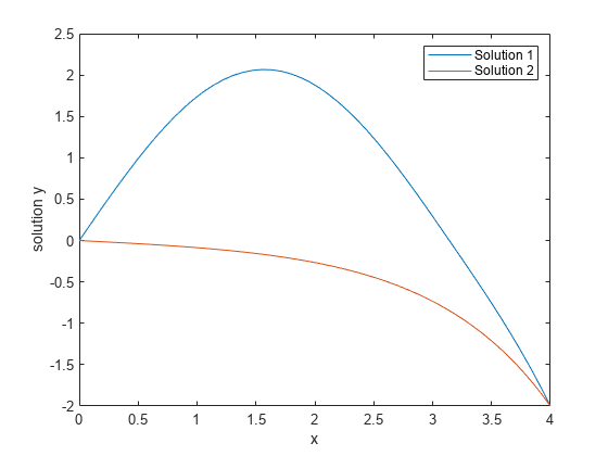
This particular boundary value problem has exactly two solutions. You can obtain the other solution by changing the initial guesses to $y （（ X ） = - 1$ and $是的（（ X ） = 0$ 。

solinit = bvpinit([0 1 2 3 4],[-1; 0]); sol = bvp4c(@twoode,@twobc,solinit); xint = linspace(0,4,50); yint = deval(sol,xint); plot(xint,yint(1,:)); legend('Solution 1'，，，，'Solution 2'）holdoff

图包含一个轴对象。轴对象包含2个类型行的对象。这些对象代表解决方案1，解决方案2。

Delay Differential Equations

dde23，，，，ddesd，，，，andddensdsolve delay differential equations with various delays. The examplesDDEX1，，，，DDEX2，，，，DDEX3，，，，DDEX4，，，，andDDEX5form a mini tutorial on using these solvers.

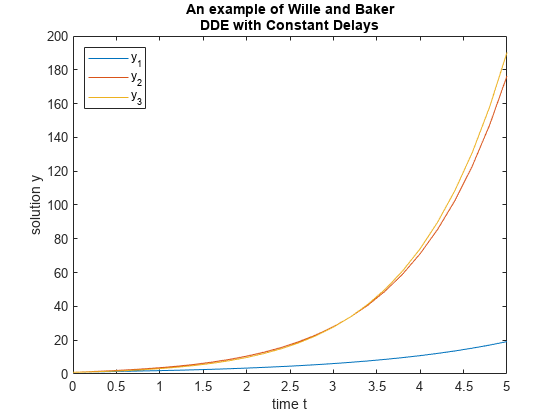
这DDEX1示例显示了如何求解微分方程的系统

$\begin{array}{l} y_{1}^{'} （（ t ） = y_{1} （（ t - 1 ） \\ y_{2}^{'} （（ t ） = y_{1} （（ t - 1 ） + y_{2} （（ t - 0 。 2 ） \\ y_{3}^{'} （（ t ） = y_{2} （（ t ）。 \end{array}$

您可以用匿名函数表示这些方程

ddex1fun = @（t，y，z）[z（1,1）;z（1,1）+z（2,2）;y（2）];

这history of the problem (for $t \leq 0$ ）is constant:

$\begin{array}{l} y_{1} （（ t ） = 1 \\ y_{2} （（ t ） = 1 \\ y_{3} （（ t ） = 1 。 \end{array}$

您可以表示历史记录为矢量。

ddex1hist =一个（3,1）;

A two-element vector represents the delays in the system of equations.

lags = [1 0.2];

Pass the function, delays, solution history, and interval of integration $[[0 ，，，， 5 这是给予的$ to the solver as inputs. The solver produces a continuous solution over the whole interval of integration that is suitable for plotting.

sol = dde23（ddex1fun，lags，ddex1hist，[0 5]）;情节（sol.x，sol.y）;标题（{'An example of Wille and Baker'，，，，'DDE持续延迟'}）;Xlabel（'时间t'）；ylabel（'solution y'）；legend('y_1'，，，，'y_2'，，，，'y_3'，，，，'Location'，，，，'西北'）；

图包含一个轴对象。带有标题的轴对象是Wille和Baker DDE带有常数延迟的示例，包含3个类型行的对象。这些对象代表y_1，y_2，y_3。

部分微分方程

pdepe在一个空间变量和时间中求解部分微分方程。示例pdex1，，，，pdex2，，，，pdex3，，，，pdex4，，，，andpdex5form a mini tutorial on usingpdepe。

This example problem uses the functionspdex1pde，，，，pdex1ic，，，，andPDEX1BC。

pdex1pde定义微分方程

$π^{2} \frac{\partial 你}{\partial t} = \frac{\partial}{\partial X} （（ \frac{\partial 你}{\partial X} ）。$

类型pdex1pde

function [c,f,s] = pdex1pde(x,t,u,DuDx) %PDEX1PDE Evaluate the differential equations components for the PDEX1 problem. % % See also PDEPE, PDEX1. % Lawrence F. Shampine and Jacek Kierzenka % Copyright 1984-2014 The MathWorks, Inc. c = pi^2; f = DuDx; s = 0;

pdex1icsets up the initial condition

$你（（ X ，，，， 0 ） = 罪 π X 。$

类型pdex1ic

function u0 = pdex1ic(x) %PDEX1IC Evaluate the initial conditions for the problem coded in PDEX1. % % See also PDEPE, PDEX1. % Lawrence F. Shampine and Jacek Kierzenka % Copyright 1984-2014 The MathWorks, Inc. u0 = sin(pi*x);

PDEX1BC设置边界条件

$你（（ 0 ，，，， t ） = 0 ，，，，$

$π e^{- t} + \frac{\partial}{\partial X} 你（（ 1 ，，，， t ） = 0 。$

类型PDEX1BC

函数[PL，QL，PR，QR] = PDEX1BC（XL，UL，XR，UR，T）％PDEX1BC评估PDEX1中编码的问题的边界条件。％％另请参见PDEPE，PDEX1。％Lawrence F. Shampine和Jacek Kierzenka％版权1984-2014 The Mathworks，Inc。pl = ul;ql = 0;pr = pi * exp（-t）;QR = 1;

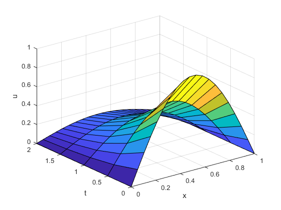
pdeperequires the spatial discretizationXand a vector of timest（在其中您想要该解决方案的快照）。使用20个节点的网格解决问题，并在五个值中要求解决方案t。Extract and plot the first component of the solution.

X=linspace(0,1,20); t = [0 0.5 1 1.5 2]; sol = pdepe(0,@pdex1pde,@pdex1ic,@pdex1bc,x,t); u1 = sol(:,:,1); surf(x,t,u1); xlabel('X'）；ylabel（'t'）；Zlabel（'U'）；

图包含一个轴对象。轴对象包含类型表面的对象。

也可以看看

ode45|bvp4c|pdepe