Generate Random Numbers Using the Triangular Distribution
This example shows how to create a triangular probability distribution object based on sample data, and generate random numbers for use in a simulation.
Step 1. Input sample data.
Input the data vectortime, which contains the observed length of time (in seconds) that 10 different cars stopped at a highway tollbooth.
time = [6 14 8 7 16 8 23 6 7 15];
The data shows that, while most cars stopped for 6 to 16 seconds, one outlier stopped for 23 seconds.
Step 2. Estimate distribution parameters.
Estimate the triangular distribution parameters from the sample data.
lower = min(time); peak = median(time); upper = max(time);
A triangular distribution provides a simplistic representation of the probability distribution when sample data is limited. Estimate the lower and upper boundaries of the distribution by finding the minimum and maximum values of the sample data. For the peak parameter, the median might provide a better estimate of the mode than the mean, since the data includes an outlier.
Step 3. Create a probability distribution object.
Create a triangular probability distribution object using the estimated parameter values.
pd = makedist('Triangular','a',lower,'b',peak,'c',upper)
pd = TriangularDistribution A = 6, B = 8, C = 23
Compute and plot the pdf of the triangular distribution.
x = 0:.1:230; y = pdf(pd,x); plot(x,y) title('Time Spent at Tollbooth') xlabel('Time (seconds)') xlim([0 30])
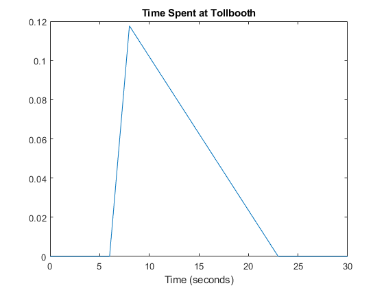
The plot shows that this triangular distribution is skewed to the right. However, since the estimated peak value is the sample median, the distribution should be symmetrical about the peak. Because of its skew, this model might, for example, generate random numbers that seem unusually high when compared to the initial sample data.
Step 4. Generate random numbers.
Generate random numbers from this distribution to simulate future traffic flow through the tollbooth.
rng('default');% For reproducibilityr = random(pd,10,1)
r =10×116.1265 18.0987 8.0796 18.3001 13.3176 7.8211 9.4360 12.2508 19.7082 20.0078
The returned values inrare the time in seconds that the next 10 simulated cars spend at the tollbooth. These values seem high compared to the values in the original data vectortimebecause the outlier skewed the distribution to the right. Using the second-highest value as the upper limit parameter might mitigate the effects of the outlier and generate a set of random numbers more similar to the initial sample data.
Step 5. Revise estimated parameters.
Estimate the upper boundary of the distribution using the second largest value in the sample data.
sort_time = sort(time,'descend'); secondLargest = sort_time(2);
Step 6. Create a new distribution object and plot the pdf.
创建一个新的特里安gular probability distribution object using the revised estimated parameters, and plot its pdf.
figure pd2 = makedist('Triangular','a',lower,'b',peak,'c',secondLargest); y2 = pdf(pd2,x); plot(x,y2,'LineWidth',2) title('Time Spent at Tollbooth') xlabel('Time (seconds)') xlim([0 30])
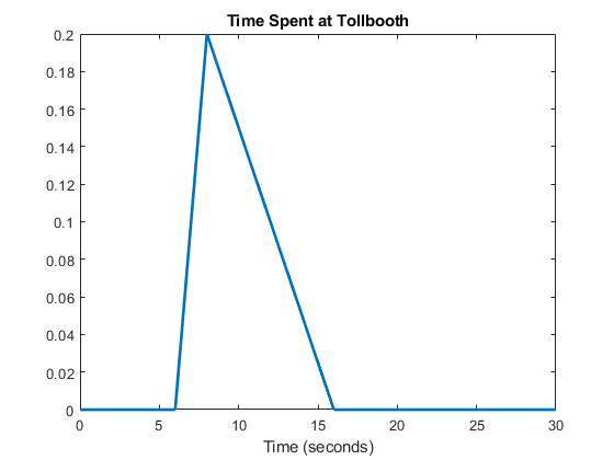
The plot shows that this triangular distribution is still slightly skewed to the right. However, it is much more symmetrical about the peak than the distribution that used the maximum sample data value to estimate the upper limit.
Step 7. Generate new random numbers.
Generate new random numbers from the revised distribution.
rng('default');% For reproducibilityr2 = random(pd2,10,1)
r2 =10×112.1501 13.2547 7.5937 13.3675 10.5768 7.3967 8.4026 9.9792 14.1562 14.3240
These new values more closely resemble those in the original data vectortime. They are also closer to the sample median than the random numbers generated by the distribution that used the outlier to estimate its upper limit. This example does not remove the outlier from the sample data when computing the median. Other options for parameter estimation include removing outliers from the sample data altogether, or using the mean or mode of the sample data as the peak value.
See Also
Related Topics
Select a Web Site
Choose a web site to get translated content where available and see local events and offers. Based on your location, we recommend that you select:.
Selectweb siteYou can also select a web site from the following list:
Americas
- América Latina(Español)
- Canada(English)
- United States(English)
Europe
- Belgium(English)
- Denmark(English)
- Deutschland(Deutsch)
- España(Español)
- Finland(English)
- France(Français)
- Ireland(English)
- Italia(Italiano)
- Luxembourg(English)
- Netherlands(English)
- Norway(English)
- Österreich(Deutsch)
- Portugal(English)
- Sweden(English)
- Switzerland
- United Kingdom(English)