Visualizing RF Budget Analysis over Bandwidth
This example shows how to programmatically perform an RF budget analysis of an RF receiver system and visualize the computed budget results across the bandwidth of the input signal.
First, useamplifier,modulator,rfelement, andnportobjects to specify the 2-port RF elements in a design. Then compute RF budget results by cascading the elements together into an RF system withrfbudget.
Therfbudgetobject enables design exploration and visualization at the MATLAB® command-line or graphically in theRF Budget Analyzerapp. It also enables automatic RF Blockset™ model and measurement testbench generation.
Introduction
RF system designers typically begin a design process with budget specifications for the gain, noise figure (NF), and nonlinearity (IP3) of the entire system.
MATLAB functionality supporting RF budget analysis makes it easy to visualize gain, NF and IP3 results at multiple frequencies throughout the bandwidth of the signal. You can:
Programmatically build an
rfbudgetobject out of 2-port RF elements.Use the Command Line display of the
rfbudgetobject to view single-frequency budget results.Vectorize the input frequency of the
rfbudgetobject and use MATLAB plot to visualize RF budget results across the bandwidth of the input signal.
In addition, with anrfbudgetobject you can:
Use export methods to generate MATLAB scripts, RF Blockset models, or measurement testbenches in Simulink®.
Use
showcommand to copy anrfbudgetobject into theRF Budget Analyzerapp.
Building Elements of RF Receiver
A basic RF receiver consists of an RF filter, an RF amplifier, a demodulator, an IF filter, and an IF amplifier.
First build and parameterize each of the 2-port RF elements. Then userfbudgetto cascade the elements with input frequency 2.1 GHz, input power -30 dBm, and input bandwidth 45 MHz.
f1 = nport('RFBudget_RF.s2p','RFBandpassFilter'); a1 = amplifier('Name','RFAmplifier',...'Gain',11.53,...'NF',1.53,...'OIP3',35); d = modulator('Name','Demodulator',...'Gain',-6,...'NF',4,...'OIP3',50,...'LO',2.03e9,...'ConverterType','Down'); f2 = nport('RFBudget_IF.s2p','IFBandpassFilter'); a2 = amplifier('Name','IFAmplifier',...'Gain',30,...'NF',8,...'OIP3',37); b = rfbudget('Elements',[f1 a1 d f2 a2],...'InputFrequency',2.1e9,...'AvailableInputPower',-30,...'SignalBandwidth',45e6);
Visualize RF Budget Results in MATLAB
Scalar frequency results can be viewed simply by using MATLABdispto see the results at the Command Line. Each column of the budget shows the results of cascading only the elements of the previous columns. Note that final column shows the RF budget results of the entire cascade.
disp(b)
rfbudget with properties: Elements: [1x5 rf.internal.rfbudget.Element] InputFrequency: 2.1 GHz AvailableInputPower: -30 dBm SignalBandwidth: 45 MHz Solver: Friis AutoUpdate: true Analysis Results OutputFrequency: (GHz) [ 2.1 2.1 0.07 0.07 0.07] OutputPower: (dBm) [-31.53 -20 -26 -27.15 2.847] TransducerGain: (dB) [-1.534 9.996 3.996 2.847 32.85] NF: (dB) [ 1.533 3.064 3.377 3.611 7.036] IIP2: (dBm) [] OIP2: (dBm) [] IIP3: (dBm) [ Inf 25 24.97 24.97 4.116] OIP3: (dBm) [ Inf 35 28.97 27.82 36.96] SNR: (dB) [ 65.91 64.38 64.07 63.83 60.41]
Plot RF Budget Results Versus Input Frequency
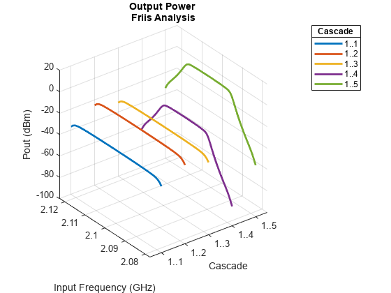
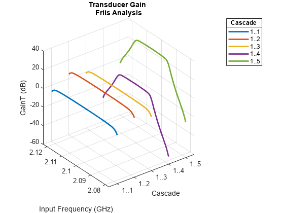
Use the budget'srfplotfunction to produce report-ready plots of cumulative RF budget results versus a range of cascade input frequencies. Cumulative (i.e. terminated sub-cascade) results are automatically computed to show the variation of the RF budget result through the entire design. Use the data cursor of the figure window to interactively explore values at different frequencies at different stages.
rfplot(b,'Pout')
rfplot(b,'GainT')
Plot RF Budget Network Parameter Results Versus Input Frequency
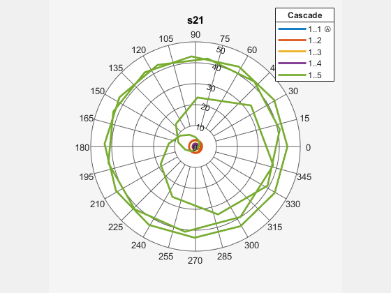
Use the RF budgetsmithplot/polarfunction to produce plots of cumulative RF budget sparameter results versus a range of cascade input frequencies. Usesmithplotfunction to view reflection coefficients and polar to view reflection and transmission coefficients.
smithplot(b,1,1)

polar(b,2,1)
Easily Export to RF Blockset and Simulink
Therfbudgetobject has other useful MATLAB methods:
exportScript- generate a MATLAB script that builds the current designexportRFBlockset- generate an RF Blockset model for simulationexportTestbench- generate a Simulink measurement testbench
Visualize RF Budget Results in App
Use the show command to copy a single-frequencyrfbudgetobject into theRF Budget Analyzerapp. ThePlot,史密斯, andPolarbutton in the app, with its pull-down options, callsrfplot,smithplot, andpolarrespectively.
In the app, theExport button copies the current design to anrfbudgetobject in the MATLAB workspace. All of the other export methods of the RF budget object are available through the pulldown options of the Export button.
show(b)

Automatically Create Reports From MATLAB Files
If you have written a'myfile.m'script that builds your design and visualizes it withrfplotcommands, try thepublish('myfile.m')function at the command line (or click thePublishbutton in the MATLAB editor). This automatically generates all figures and produces a report for your colleagues, saved as an html file.
To save your design, first undock using the commands shown below and then use the Figure Toolbar to pulldown the File Menu and save usingFile->Save Asand select the Save as type to png or pdf. To redock the figure window into the app you can click the Dock affordance on the upper right corner of the figure window.
h = findall(0,'type','figure','name','untitled'); set(h,'WindowStyle','normal') set(h,'MenuBar','figure') set(h,'ToolBar','auto')
Related Topics
You can also select a web site from the following list:
Americas
- América Latina(Español)
- Canada(English)
- United States(English)
Europe
- Belgium(English)
- Denmark(English)
- Deutschland(Deutsch)
- España(Español)
- Finland(English)
- France(Français)
- Ireland(English)
- Italia(Italiano)
- Luxembourg(English)
- Netherlands(English)
- Norway(English)
- Österreich(Deutsch)
- Portugal(English)
- Sweden(English)
- Switzerland
- United Kingdom(English)