Monopole Measurement Comparison

Open Live Script

这个例子比较了磁单极子的阻抗analyzed in Antenna Toolbox™ with the measured results. The corresponding antenna was fabricated and measured at the Center for Metamaterials and Integrated Plasmonics (CMIP), Duke University. The monopole is designed for an operating frequency of 2.5 GHz.

Create, Modify and View Monopole

Create the default monopole antenna geometry. Then, modify the height and the width of the monopole, and dimensions of the ground plane to be in agreement with the hardware prototype. Since the monopole is located at the center of the ground plane, the FeedOffset property of the antenna is not modified.

mp = monopole; mp.Height = 28.5e-3; mp.Width = 2.54e-3; mp.GroundPlaneLength = 0.1; mp.GroundPlaneWidth = 0.1; figure; show(mp)

Figure contains an axes object. The axes object with title monopole antenna element contains 4 objects of type patch, surface. These objects represent PEC, feed.

Plot Impedance and Return Loss

定义分析的频带。的罗wer band frequency is 500 MHz and the upper band frequency is 5 GHz. Since the reference impedance is not specified as one of the arguments when calculating the return loss, the default value of 50 $Ω$ will be used.

freq = 0.5e9:50e6:5e9; RL = returnLoss(mp,freq); [~,ind1] = max(RL); figure; impedance(mp,freq); marker1 = linspace(-500,500,21); holdonplot(freq(ind1).*ones(1,21)./1e9,marker1,'m-.','LineWidth',2) textInfo = [' \leftarrow'num2str(freq(ind1)/1e9)'GHz']; text(freq(ind1-1)/1e9,300,textInfo,'FontSize',11) holdoff

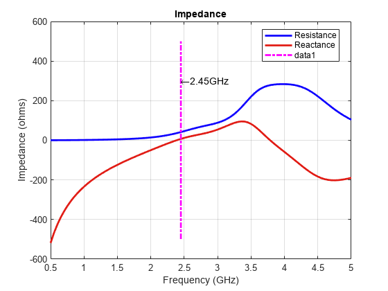
Figure contains an axes object. The axes object with title Impedance contains 4 objects of type line, text. These objects represent Resistance, Reactance.

figure returnLoss(mp,freq); marker2 = linspace(0,30,21); holdonplot(freq(ind1).*ones(1,21)./1e9,marker2,'m-.','LineWidth',2) holdoff

Figure contains an axes object. The axes object with title Return Loss contains 2 objects of type line.

Comparison with Measurement - Reflection Coefficient

Measurements were taken of the fabricated monopole over the same frequency band. The measured data is the reflection coefficient % ( $S_{11}$ ) of the monopole in decibels. To compare with measurements, plot the numerical reflection coefficient, which is the negative of the return loss.

load('monopole_measured.mat'); figure; plot(freq/1e9,-mp.returnLoss(freq),'b','linewidth',3); holdon; plot(f/1e9,S11dB,'r','linewidth',3); holdoff; gridonlegend('Analysis','Measurement','Location','Best'); xlabel('Frequency (GHz)'); ylabel('S_1_1 (dB)'); title('Monopole Antenna');

Figure contains an axes object. The axes object with title Monopole Antenna contains 2 objects of type line. These objects represent Analysis, Measurement.

The figure indicates a good agreement between theory and measurements. Typically, a criterion such as $S_{11} < - 10 d B$ is used for describing a good impedance match. The analysis and measurement confirm that the monopole satisfies the criterion in a band centered about 2.5 GHz. The fabricated monopole and the measurement setup are shown below.

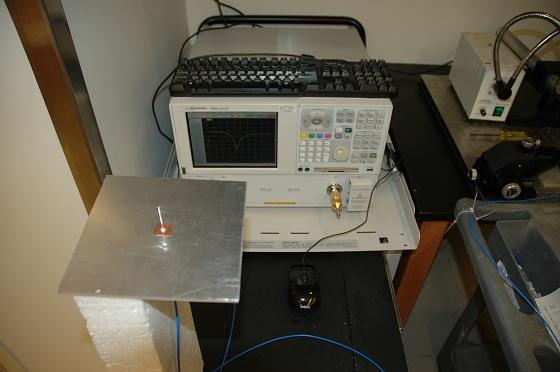
Fabricated monopole, and measurement setup (with permission from CMIP, Duke University)

Monopole Measurement Comparison

Create, Modify and View Monopole

Plot Impedance and Return Loss

Comparison with Measurement - Reflection Coefficient

See Also