問題ベースの最適化の出力関数

この例では、出力関数を使用してプロットし、非線形問題の反復の履歴を保存する方法を説明します。この履歴には、評価点、ソルバーが点の生成に使用する探索方向、評価点での目的関数値が含まれます。

この例へのソルバーベースのアプローチについては、Optimization Toolbox™ の出力関数を参照してください。

プロット関数の構文は出力関数と同じであるため、この例はプロット関数にも適用されます。

ソルバーベースのアプローチと問題ベースのアプローチの両方で、ソルバーベースのアプローチと同様に出力関数を記述します。ソルバーベースのアプローチでは、単一のベクトル変数を使用します。この変数は通常、さまざまなサイズの最適化変数の集合ではなく、xと表されます。そのため、問題ベースのアプローチの出力関数を記述するには、最適化変数と単一のソルバーベースのxとの間の対応を理解しなければなりません。最適化変数とxとの間でマッピングを行うには、varindexを使用します。この例では、xという名前の最適化変数との混同を避けるために、in"をベクトル変数名として使用します。

問題の説明

この問題では、変数xおよびyの次の関数を最小化します。

$f = \exp (x) (4 x^{2} + 2 y^{2} + 4 x y + 2 y + 1) .$

さらに、この問題には 2 つの非線形制約があります。

$\begin{array}{l} x + y - x y \geq 1.5 \\ x y \geq - 10 . \end{array}$

問題ベースの設定

問題ベースのアプローチで問題を設定するには、最適化変数と最適化問題オブジェクトを定義します。

x = optimvar('x'); y = optimvar('y'); prob = optimproblem;

最適化変数の式として目的関数を定義します。

f = exp(x)*(4*x^2 + 2*y^2 + 4*x*y + 2*y + 1);

目的関数をprobに含めます。

prob.Objective = f;

非線形制約を含めるには、最適化制約式を作成します。

cons1 = x + y - x*y >= 1.5; cons2 = x*y >= -10; prob.Constraints.cons1 = cons1; prob.Constraints.cons2 = cons2;

これは非線形問題であるため、初期点構造体x0を含めなければなりません。x0.x = –1およびx0.y = 1を使用します。

x0.x = -1; x0.y = 1;

出力関数

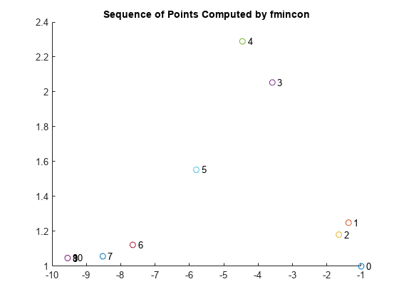
出力関数outfunは、その反復中にfminconによって生成される点の履歴を記録します。出力関数はさらに点をプロットし、sqpアルゴリズムの探索方向の別の履歴を保持します。探索方向は、前の点からfminconが試みる次の点へのベクトルです。最終ステップでは、出力関数がワークスペース変数に履歴を保存し、反復ステップごとに目的関数値の履歴を保存します。

必要となる最適化出力関数の構文については、出力関数とプロット関数の構文を参照してください。

出力関数は単一のベクトル変数を入力として取ります。しかし、現在の問題には 2 つの変数があります。最適化変数と入力変数の間のマッピングを確認するには、varindexを使用します。

idx = varindex(prob); idx.x

ans = 1

idx.y

ans = 2

マッピングは,xが変数 1 でyが変数 2 であることを示しています。そのため、入力変数の名前がinである場合、x = in(1)およびy = in(2)になります。

typeoutfun

function stop = outfun(in,optimValues,state,idx) persistent history searchdir fhistory stop = false; switch state case 'init' hold on history = []; fhistory = []; searchdir = []; case 'iter' % Concatenate current point and objective function % value with history. in must be a row vector. fhistory = [fhistory; optimValues.fval]; history = [history; in(:)']; % Ensure in is a row vector % Concatenate current search direction with % searchdir. searchdir = [searchdir;... optimValues.searchdirection(:)']; plot(in(idx.x),in(idx.y),'o'); % Label points with iteration number and add title. % Add .15 to idx.x to separate label from plotted 'o' text(in(idx.x)+.15,in(idx.y),... num2str(optimValues.iteration)); title('Sequence of Points Computed by fmincon'); case 'done' hold off assignin('base','optimhistory',history); assignin('base','searchdirhistory',searchdir); assignin('base','functionhistory',fhistory); otherwise end end

OutputFcnオプションを設定して、最適化に出力関数を含めます。また、既定の'interior-point'アルゴリズムではなく'sqp'アルゴリズムを使用するようにAlgorithmオプションを設定します。idxを最後の入力の追加パラメーターとして出力関数に渡します。詳細は、追加パラメーターの受け渡しを参照してください。

outputfn = @(in,optimValues,state)outfun(in,optimValues,state,idx); opts = optimoptions(“fmincon”,'Algorithm','sqp','OutputFcn',outputfn);

出力関数を使用した最適化の実行

名前と値のペアの引数 'Options'を使用して、出力関数を含む最適化を実行します。

[sol,fval,eflag,output] = solve(prob,x0,'Options',opts)

Solving problem using fmincon.

Figure contains an axes object. The axes object with title Sequence of Points Computed by fmincon contains 22 objects of type line, text.

Local minimum found that satisfies the constraints. Optimization completed because the objective function is non-decreasing in feasible directions, to within the value of the optimality tolerance, and constraints are satisfied to within the value of the constraint tolerance.

sol =struct with fields:x: -9.5474 y: 1.0474

fval = 0.0236

eflag = OptimalSolution

output =struct with fields:iterations: 10 funcCount: 22 algorithm: 'sqp' message: '...' constrviolation: 1.2434e-14 stepsize: 1.4785e-07 lssteplength: 1 firstorderopt: 7.1930e-10 bestfeasible: [1x1 struct] objectivederivative: "reverse-AD" constraintderivative: "closed-form" solver: 'fmincon'

反復の履歴を確認します。行列optimhistoryの各行は 1 つの点を表します。最後のいくつかの点は非常に近接しています。そのため、シーケンスのプロットには点 8、9、10 を示す数が重なって表示されています。

disp('Locations');disp(optimhistory)

Locations -1.0000 1.0000 -1.3679 1.2500 -1.6509 1.1813 -3.5870 2.0537 -4.4574 2.2895 -5.8015 1.5531 -7.6498 1.1225 -8.5223 1.0572 -9.5463 1.0464 -9.5474 1.0474 -9.5474 1.0474

配列searchdirhistoryおよびfunctionhistoryを確認します。

disp('Search Directions');disp(searchdirhistory)

Search Directions 0 0 -0.3679 0.2500 -0.2831 -0.0687 -1.9360 0.8725 -0.8704 0.2358 -1.3441 -0.7364 -2.0877 -0.6493 -0.8725 -0.0653 -1.0241 -0.0108 -0.0011 0.0010 0.0000 -0.0000

disp('Function Values');disp(functionhistory)

Function Values 1.8394 1.8513 1.7757 0.9839 0.6343 0.3250 0.0978 0.0517 0.0236 0.0236 0.0236

`fcn2optimexpr`を必要とするサポートされていない関数

目的関数または非線形制約関数が初等関数で構成されていない場合,fcn2optimexprを使用して、その関数を最適化式に変換しなければなりません。詳細は、非線形関数から最適化式への変換を参照してください。この例では、次のコードを入力します。

fun = @(x,y)exp(x)*(4*x^2 + 2*y^2 + 4*x*y + 2*y + 1); f = fcn2optimexpr(fun,x,y);

サポートされている関数の一覧については、最適化変数および式でサポートされる演算を参照してください。

参考

varindex