拟合利率曲线功能

This example uses:

Open Live Script

This example shows how to useIRFunctionCurve对象建模利率的术语结构（也称为收益曲线）。这可以与对术语结构进行建模与日期和数据的向量进行建模，并在点之间进行插值（目前可以使用函数来完成prbyzero). The term structure can refer to at least three different curves: the discount curve, zero curve, or forward curve.

TheIRFunctionCurveobject allows you to model an interest-rate curve as a function.

This example explores using anIRFunctionCurveobject to model the default-free term structure of interest rates in the United Kingdom. Three different forms for the term structure are implemented and are discussed in more detail later:

Nelson-Siegel
Svensson
Smoothing Cubic Spline with a so-called Variable Roughness Penalty (VRP)

Choosing the Data

The first question in modeling the yield curve is what data should be used. To model a default-free yield curve, default-free, option-free market instruments must be used. The most significant component of the data is UK Government Bonds (known as Gilts). Historical data is retrieved from the following site:

https://www.dmo.gov.uk

Repo data is used to construct the short end of the yield curve. Repo data is retrieved from the following site:

https://www.ukfinance.org.uk/

Note also that the data must be specified as a matrix where the columns areSettle,Maturity,CleanPrice, andCouponRateand that instruments must be bonds or synthetically converted to bonds.

Market data for a close date of April 30, 2008, has been downloaded and saved to the following data file (ukdata20080430), which is loaded into MATLAB® with the following command:

%加载数据loadukdata20080430% Convert repo rates to be equivalent zero coupon bondsRepoCouponRate = repmat(0,size(RepoRates)); RepoPrice = bndprice(RepoRates, RepoCouponRate, RepoSettle, RepoMaturity);% Aggregate the dataSettle = [RepoSettle;BondSettle]; Maturity = [RepoMaturity;BondMaturity]; CleanPrice = [RepoPrice;BondCleanPrice]; CouponRate = [RepoCouponRate;BondCouponRate]; Instruments = [Settle Maturity CleanPrice CouponRate]; InstrumentPeriod = [repmat(0,6,1);repmat(2,31,1)]; CurveSettle = datenum('30-Apr-2008');

Fit Nelson-Siegel Model to Market Data

The Nelson-Siegel model proposes that the instantaneous forward curve can be modeled with the following:

$f = β_{0} + β_{1} e^{\frac{- m}{τ}} + β_{2} e^{\frac{- m}{τ}} \frac{m}{τ}$

This can be integrated to derive an equation for the zero curve (see [6] for more information on the equations and the derivation):

$s = β_{0} + (β_{1} + β_{2}) \frac{τ}{m} (1 - e^{\frac{- m}{τ}}) - β_{2} e^{\frac{- m}{τ}}$

See [1] for more information.

TheIRFunctionCurveobject provides the capability to fit a Nelson Siegel curve to observed market data with thefitNelsonSiegelmethod. The fitting is done by calling the Optimization Toolbox™ functionlsqnonlin.

ThefitNelsonSiegelfunction has required inputs for CurveType, CurveSettle, and a matrix of instrument data.

Optional input arguments, specified in name-value pair argument, are:

IRFitOptionsstructure: Provides the capability to choose which quantity to be minimized (price, yield, or duration weighted price) and other optimization parameters (for example, upper and lower bounds for parameters).
CurveCompoundingandBasis(day-count convention)
Additional instrument parameters,Period,Basis,FirstCouponDate, and so on.

NSModel = IRFunctionCurve.fitNelsonSiegel('Zero',CurveSettle,...Instruments,'InstrumentPeriod',InstrumentPeriod);

Fit Svensson Model

一个非常类似的模型- siegel模型the Svensson model, which adds two additional parameters to account for greater flexibility in the term structure. This model proposes that the forward rate can be modeled with the following form:

$f = β_{0} + β_{1} e^{\frac{- m}{τ_{1}}} + β_{2} e^{\frac{- m}{τ_{1}}} \frac{m}{τ_{1}} + β_{3} e^{\frac{- m}{τ_{2}}} \frac{m}{τ_{2}}$

As above, this can be integrated to derive an equation for the zero curve:

$s = β_{0} + β_{1} (1 - e^{\frac{- m}{τ_{1}}}) (- \frac{τ_{1}}{m}) + β_{2} ((1 - e^{\frac{- m}{τ_{1}}}) \frac{τ_{1}}{m} - e^{\frac{m}{τ_{1}}}) + β_{3} ((1 - e^{\frac{- m}{τ_{2}}}) \frac{τ_{2}}{m} - e^{\frac{m}{τ_{2}}})$

See [2] for more information.

Fitting the parameters to this model proceeds in a similar fashion to the Nelson-Siegel model using thefitSvenssonfunction.

SvenssonModel = IRFunctionCurve.fitSvensson('Zero',CurveSettle,...Instruments,'InstrumentPeriod',InstrumentPeriod);

Fit Smoothing Spline

The term structure can also be modeled with a spline, specifically, one way to model the term structure is by representing the forward curve with a cubic spline. To ensure that the spline is sufficiently smooth, a penalty is imposed relating to the curvature (second derivative) of the spline:

$\sum_{i = 1}^{N} [\frac{P_{i} - {P_{}^{ˆ}}_{i} (f)}{D_{i}}]^{2} + \int_{0}^{M} λ_{t} (m) [f^{''} (m)]^{2} d m$

where the first term is the difference between the observed pricePand the predicted price,P_hat, (weighted by the bond's duration,D) summed over all bonds in the data set, and the second term is the penalty term (wherelambdais a penalty function andfis the spline).

See [3], [4], [5] below.

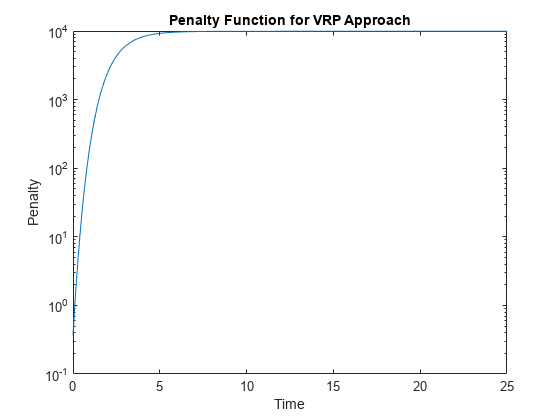
There have been different proposals for the specification of the penalty functionlambda. One approach, advocated by [4], and currently used by the UK Debt Management Office, is a penalty function of the following form:

$l o g (λ (m)) = L - (L - S) e^{\frac{- m}{μ}}$

The parametersL,S, andmuare typically estimated from historical data.

TheIRFunctionCurveobject can be used to fit a smoothing spline representation of the forward curve with a penalty function using the functionfitSmoothingSpline.

Required inputs, like for the functions above, are aCurveType, CurveSettle,Instrumentsmatrix, and a function handle (Lambdafun) containing the penalty function.

The optional parameters are similar tofitNelsonSiegelandfitSvensson.

% Parameters chosen to be roughly similar to [4] below.L = 9.2; S = -1; mu = 1; lambdafun = @(t) exp(L - (L-S)*exp(-t/mu));% Construct penalty functiont = 0:.1:25;% Construct data to plot penalty functiony = lambdafun(t); figure semilogy(t,y); title('Penalty Function for VRP Approach') ylabel('Penalty'）xlabel（'Time')

Figure contains an axes object. The axes object with title Penalty Function for VRP Approach contains an object of type line.

VRPModel = IRFunctionCurve.fitSmoothingSpline('Forward',CurveSettle,...乐器，兰巴芬，'Compounding',-1,...'InstrumentPeriod',InstrumentPeriod);

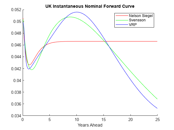
Use Fitted Curves and Plot Results

Once a curve is created, functions are used to extract the Forward and Zero Rates and the Discount Factors. This curve can also be converted into aRatesspecstructure using thetoRateSpecfunction. TheRatesspeccan then be used with many other functions in the Financial Instruments Toolbox™

PlottingDates = CurveSettle+20:30:CurveSettle+365*25; TimeToMaturity = yearfrac(CurveSettle,PlottingDates); NSForwardRates = NSModel.getForwardRates(PlottingDates); SvenssonForwardRates = SvenssonModel.getForwardRates(PlottingDates); VRPForwardRates = VRPModel.getForwardRates(PlottingDates); figure hold上plot(TimeToMaturity,NSForwardRates,'r') plot(TimeToMaturity,SvenssonForwardRates,'g') plot(TimeToMaturity,VRPForwardRates,'b') title('UK Instantaneous Nominal Forward Curve'）xlabel（'Years Ahead') legend({'Nelson Siegel','Svensson','VRP'})

Figure contains an axes object. The axes object with title UK Instantaneous Nominal Forward Curve contains 3 objects of type line. These objects represent Nelson Siegel, Svensson, VRP.

Compare with this Link

This link provides a live look at the derived yield curve published by the UK

https://www.bankofengland.co.uk

Bibliography

This example is based on the following papers and journal articles:

[1] Nelson, C.R., Siegel, A.F. "Parsimonious Modelling of Yield Curves."Journal of Business.60, pp 473-89, 1987.

[2] Svensson, L.E.O. "Estimating and Interpreting Forward Interest Rates: Sweden 1992-4." International Monetary Fund, IMF Working Paper, 1994/114, 1994.

[3] Fisher, M., Nychka, D., Zervos, D. "Fitting the Term Structure of Interest Rates with Smoothing Splines." Board of Governors of the Federal Reserve System, Federal Reserve Board Working Paper, 95-1, 1995.

[4] Anderson, N., Sleath, J. "New Estimates of the UK Real and Nominal Yield Curves."英格兰银行季度公告。1999年11月,页384 - 92。

[5] Waggoner, D. "Spline Methods for Extracting Interest Rate Curves from Coupon Bond Prices." Federal Reserve Board Working Paper, 97-10, 1997.

[6] "Zero-Coupon Yield Curves: Technical Documentation." BIS Papers No. 25, October 2005.

[7] Bolder，D.J.，Gusba，s。“指数，多项式和傅立叶系列：加拿大银行的更多产量曲线建模。”工作论文02-29，加拿大银行，2002年。

[8] Bolder, D.J., Streliski, D. "Yield Curve Modelling at the Bank of Canada." Technical Reports 84, Bank of Canada, 1999.