Frequency Response Specification and Filter Design

Filter responses are usually specified by frequency intervals (bands) along with the desired gain on each band. Custom magnitude and phase filter specifications are similar, but also include phase response, usually as a complex value encoding both gain and phase response. In most

cases, the response specification is comprised of a frequencies vectorF= [f1, ..., fN] ofNincreasing frequencies, and a frequency responses vectorH= [h1, ..., hN] corresponding to the filter's complex response values. In DSP System Toolbox™, you can create a filter specification object with a desired frequency response usingfdesign.arbmagnphase. Once a specification object has been created, you can design an FIR or an IIR filter using thedesignfunction. For more information about FIR and IIR design algorithms, see[1].

FIR Designs

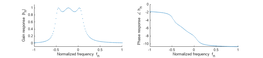
In this first example, we compare several FIR design methods to model the magnitude and phase of a complex RF bandpass filter. First, load the desired filter specification: frequencies to the vectorF,复杂的响应值向量H. Plot the gain and phase frequency responses on the the left and the right graphs respectively.

load('gainAndPhase','F','H')% Load frequency response dataplotResponse(F, H)%傅一个辅助绘图nction used in this demo

Create a specification object usingfdesign.arbmagnphasewith the'N,F,H'specification pattern. This specification accepts the desired filter orderN, along with the frequency response vectorsFandH. The'N,F,H'pattern defines the desired response on the entire Nyquist range (that is, a single-band specification with no relaxed "don't care" regions). In this example, the desired response data vectorsFandHhave 655 points, which is relatively dense across the frequency domain.

N = 100; f = fdesign.arbmagnphase('N,F,H', N,F,H);

Determine which design methods can be used for this specification object using thedesignmethodsfunction. In this case, the methods are:equiripple,firls(least squares), andfreqsamp(frequency sampling).

designmethods(f,'fir')

FIR Design Methods for class fdesign.arbmagnphase (N,F,H): equiripple firls freqsamp

Design the filters with thedesignfunction using the desired method from the list above. You can also specify'allfir'使用所有可用的方法来设计,case the function returns a cell array of System objects.

Hd = design(f,'allfir', SystemObject = true);

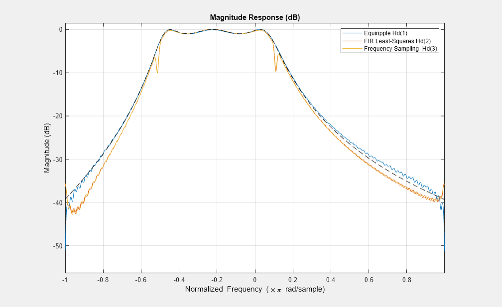
Plot the filters' frequency responses and the nominal response in a dashed line. The equiripple designHd(1)appears to approximate very well on the passband, but slightly deviates in other regions. The least squares designHd(2)is optimized for uniformly weighted quadratic norm (not favoring one region or another), and the frequency sampled FIR designHd(3)appears to exhibit the worst approximation of all three.

hfvt = fvtool(Hd{:}); legend(hfvt,'Equiripple Hd(1)','FIR Least-Squares Hd(2)','Frequency Sampling Hd(3)',...位置='NorthEast') ax = hfvt.CurrentAxes; ax.NextPlot ='add'; plot(ax,F,20*log10(abs(H)),'k--')

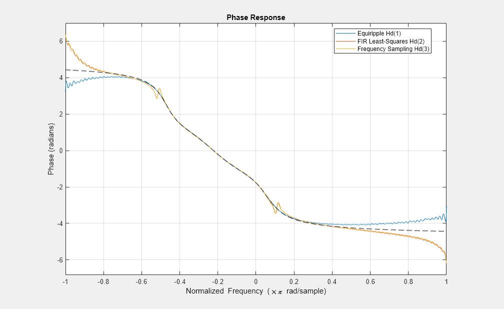
hfvt(2) = fvtool(Hd{:}, Analysis ='phase'); legend(hfvt(2),'Equiripple Hd(1)','FIR Least-Squares Hd(2)','Frequency Sampling Hd(3)') ax = hfvt(2).CurrentAxes; ax.NextPlot ='add'; plot(ax,F,unwrap(angle(H))+2*pi,'k--')

IIR Designs

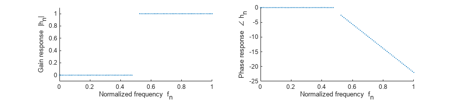
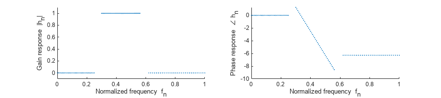
In the next part, we design an IIR filter. The desired filter is a halfband highpass filter with a linear phase on the passband. The specification is given by 100 points on the frequency domain as shown in the following figure.

F = [linspace(0,.475,50) linspace(.525,1,50)]; H = [zeros(1,50) exp(-1j*pi*13*F(51:100))]; plotResponse(F, H)

Create a specification object using a single-band design spec'Nb, Na, F, H', which takes the desired IIR ordersNa= 10(denominator order) andNb= 12(numerator order) as inputs. There is only one design method available for this specification - the least squares IIR design (iirls).

Nb = 12; Na = 10; f = fdesign.arbmagnphase('Nb,Na,F,H',Nb,Na,F,H); designmethods(f)

Design Methods for class fdesign.arbmagnphase (Nb,Na,F,H): iirls

Theiirlsdesign method allows to specify different weights for different frequencies, giving more control over the approximation quality of each band. Design the filter with a weight of 1 on the stopband and a weight of 100 on the passband. The high weight given to the passband makes the approximation more accurate on this region.

W = 1*(F<=0.5) + 100*(F>0.5); Hd = design(f,'iirls', Weights = W, SystemObject = true);

When using IIR design techniques, the stability of the filter is not guaranteed. Check the IIR stability using theisstablefunction. To do a more complete analysis, examine the poles and how close they are to the unit circle.

isstable(Hd)

ans =logical1

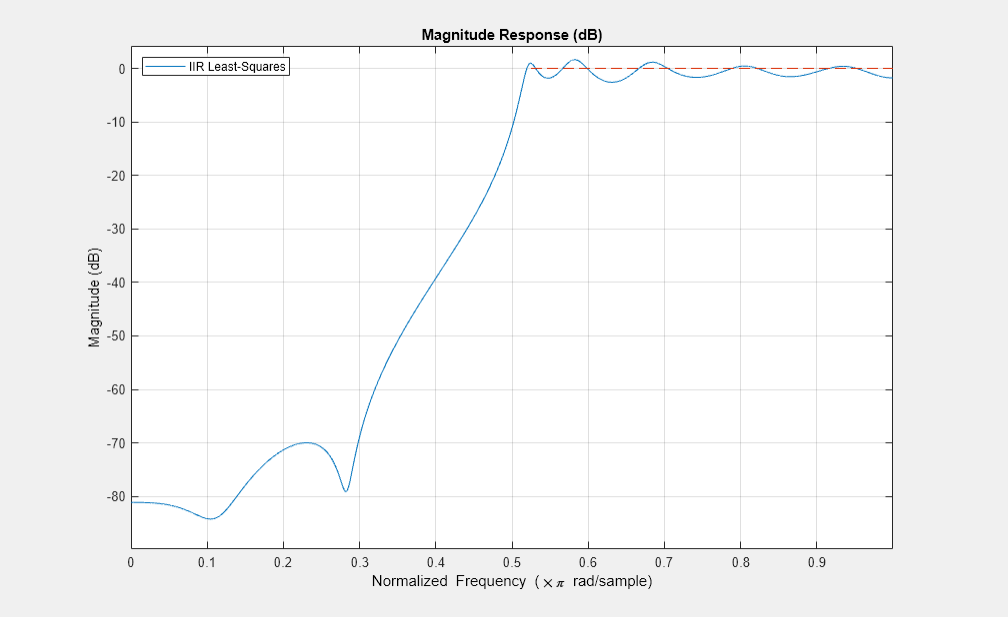
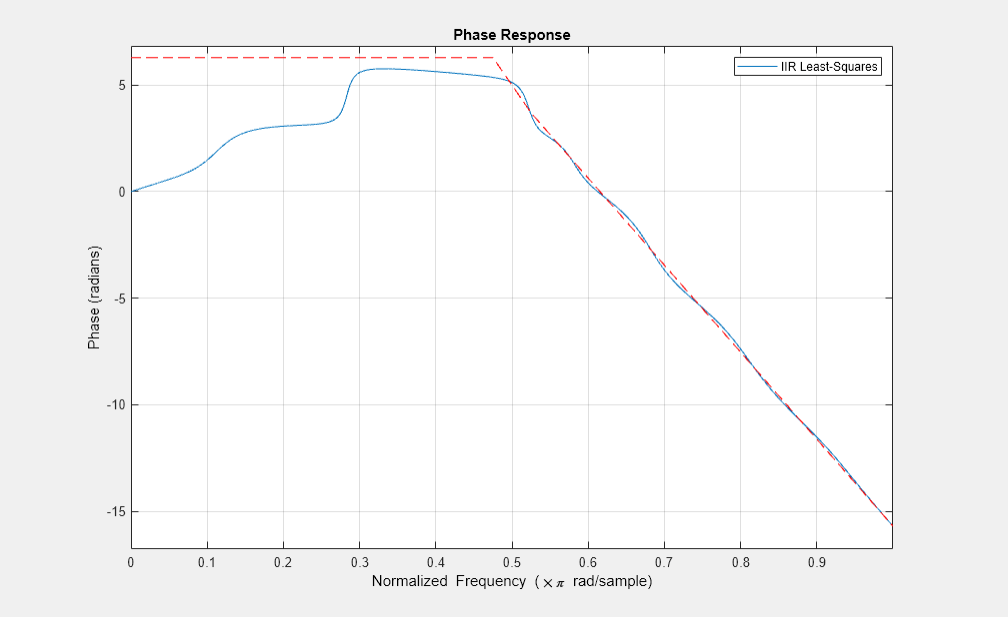
Plot the IIR design response. Note that the approximation on the passband is better than on the stopband, and the phase response is less significant wherever the magnitude gain is small (low dB).

hfvt = fvtool(Hd); legend(hfvt,'IIR Least-Squares', Location ='NorthWest')

hfvt(2) = fvtool(Hd,Analysis='phase'); legend(hfvt(2),'IIR Least-Squares', Location ='NorthEast') ax = hfvt(2).CurrentAxes; ax.NextPlot ='add'; plot(ax,F,unwrap(angle(H))+2*pi,'r--')

Bandpass FIR Design with a Low Group Delay

An interesting application of arbitrary magnitude and phase designs is the design of asymmetric FIR filters that sacrifice linear phase in favor of a shorter group delay. Such filters can still be designed to maintain a good approximation of a linear phase on the passband. Suppose we have three bands for the bandpass filter: a stopband on ${\mathit{F}}_1=[0,0.3)$and on $$F_3=(0.6,1]$$, and a passband on ${\mathit{F}}_2=\left[0.3,0.6\right]$. On the passband, the desired frequency response is $\mathit{H}\left(\omega \right)={\mathit{e}}^{-\mathit{j}\pi \omega \cdot \mathrm{gd}}$, which has a linear phase reponse with a group delay ofgd.

F1 = linspace(0,.25,30);% Lower stopbandF2 = linspace(.3,.56,40);%通频带F3 = linspace(.62,1,30);% Higher stopband% Define the desired frequency response on the bandsgd = 12;% Desired Group DelayH1 = zeros(size(F1)); H2 = exp(-1j*pi*F2*gd); H3 = zeros(size(F3)); F = [F1 F2 F3]; H = [H1 H2 H3];

Plot the desired frequency response.

plotResponse(F, H)

Create a filter specification object using the'N,B,F,H'specification pattern. Here,N= 50is the desired filter order,B= 3stands for the number of bands, followed byBpairs ofFandHvectors as before.

N = 50;% Filter OrderB = 3;% Number of bandsf = fdesign.arbmagnphase('N,B,F,H',N,B, F1,H1, F2,H2, F3,H3); Hd_mnp = design(f,'equiripple', SystemObject = true);

This design does not have a linear phase, as can be seen by calling theislinphasefunction.

islinphase(Hd_mnp)

ans =logical0

Now, create a magnitude-only filter specification usingfdesign.arbmag. The'N,B,F,A'specification pattern for this object is similar to the'N,B,F,H'specification of thefdesign.argmagnphaseobject. The difference between the two is that the complex filter responseHin'N,B,F,H'is replaced with a magnitude only (nonnegative real) responseAin'N,B,F,A'.

f_magonly = fdesign.arbmag('N,B,F,A',N,3,F1,abs(H1),F2,abs(H2),F3,abs(H3)); Hd_mo = design(f_magonly,'equiripple', SystemObject = true);

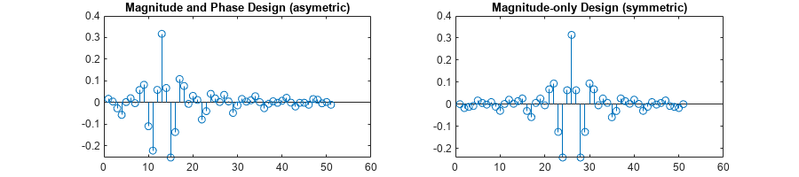
The magnitude-only specification yields symmetric design with a linear phase.

islinphase(Hd_mo)

ans =logical1

subplot(1,2,1); stem(Hd_mnp.Numerator) title('Magnitude and Phase Design (asymetric)') subplot(1,2,2); stem(Hd_mo.Numerator) title('Magnitude-only Design (symmetric)')

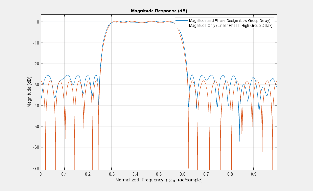
Compare the two designs. Note that they have a very similar bandpass magnitude response.

hfvt = fvtool(Hd_mnp,Hd_mo); legend(hfvt,'Magnitude and Phase Design (Low Group Delay)',...'Magnitude Only (Linear Phase, High Group Delay)', Location ='NorthEast')

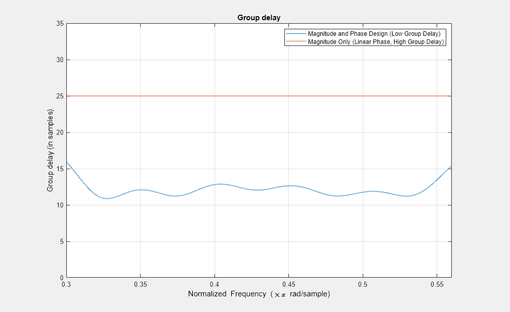
Plot the group delay. The arbitrary magnitude and phase design has a slightly varying group delay. However, the variation is small and on average is 12.5 samples. This group delay is half the group delay of the magnitude only design, which is 25 samples.

hfvt(2) = fvtool(Hd_mnp,Hd_mo, Analysis ='grpdelay'); legend(hfvt(2),'Magnitude and Phase Design (Low Group Delay)',...'Magnitude Only (Linear Phase, High Group Delay)', Location ='NorthEast') hfvt(2).zoom([.3 .56 0 35]);

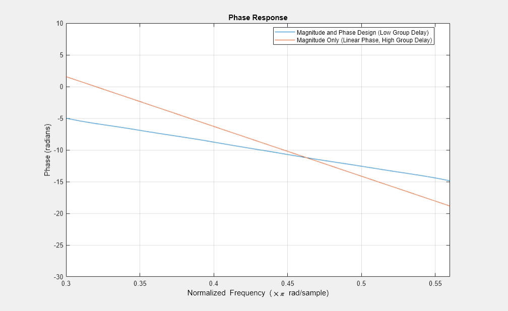
The difference in group delays can also be seen in the phase response. The shallower slope indicates a smaller group delay.

hfvt(2).Analysis ='phase'; hfvt(2).zoom([.3 .56 -30 10]);

Passband Equalization of a Chebyshev Lowpass Filter

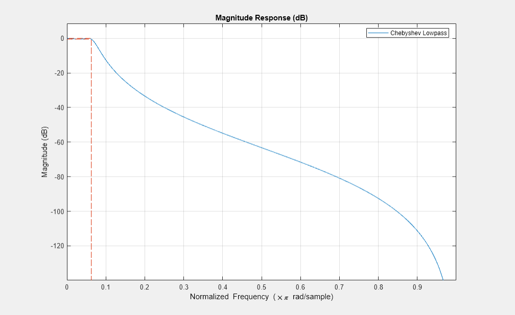
Another common application of arbitrary magnitue-phase designs is the equalization of nonlinear-phase responses of IIR filters. Consider a third order Chebyshev Type I lowpass filter with a normalized passband frequency of 1/16 and passband ripples of 0.5 dB.

Fp = 1/16;%通频带frequencyAp = .5;%通频带跑lesf = fdesign.lowpass('N,Fp,Ap',3,Fp,Ap); Hcheby = design(f,'cheby1', SystemObject = true);close(hfvt(1)); close(hfvt(2)); hfvt = fvtool(Hcheby); legend(hfvt,'Chebyshev Lowpass');

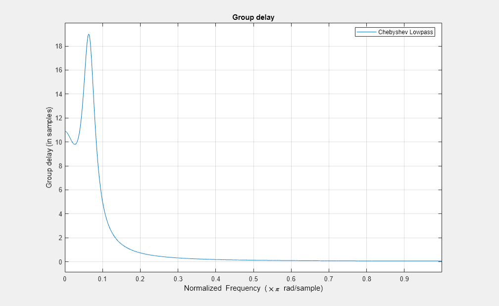
Plot the group delay. There is a significant group delay distorition on the passband with group delays ranging from 10 to 20 samples.

hfvt(2) = fvtool(Hcheby, Analysis ='grpdelay'); legend(hfvt(2),'Chebyshev Lowpass');

To mitigate the distortion in the group delay, an FIR equalizer ${\mathit{H}}_{\mathrm{eq}}\left(\omega \right)$can be used after the IIR filter. Ideally, the combined filter is an ideal lowpass. The combined filter has the passband response $\mathit{G}\left(\omega \right)={\mathit{H}}_{\mathrm{ch}}\left(\omega \right){\mathit{H}}_{\mathrm{eq}}\left(\omega \right)={\mathit{e}}^{-\mathit{j}{\mathit{g}}_{\mathit{d}}\omega }$, eliminating the magnitude ripples to a flat magnitude response and a constant group delay of ${\mathit{g}}_{\mathit{d}}$samples. The target group ${\mathit{g}}_{\mathit{d}}$is tied to the allotted FIR length for causal filter designs. In this example, ${\mathit{g}}_{\mathit{d}}=35$makes a reasonable choice.

To summarize, the equalizer design has two bands:

This two-band design specification ensures that the FIR approximation of the equalizer focuses on the passband and the stopband only. The remaining parts of the frequency domain are considered don't-care regions.

gd = 35;%通频带Group Delay of the equalized filter (linear phase)F1 = 0:5e-4:Fp;%通频带D1 = exp(-1j*gd*pi*F1)./freqz(Hcheby,F1*pi); Fst = 3/16;% StopbandF2 = linspace(Fst,1,100); D2 = zeros(1,length(F2));

There are several FIR design methods that can be used to implement this equalizer FIR specification. Compare the performance using two design methods: a least squares design, and an equiripple design.

feq = fdesign.arbmagnphase('N,B,F,H',51,2,F1,D1,F2,D2); Heq_ls = design(feq,'firls', SystemObject = true);% Least-Squares designHeq_er = design(feq,'equiripple', SystemObject = true);% Equiripple design% Create the cascaded filtersGls = cascade(Hcheby,Heq_ls); Geq = cascade(Hcheby,Heq_er);

Plot the magnitude responses of the cascaded systems for both filters.

hfvt = fvtool(Hcheby,Gls,Geq); legend(hfvt,'Chebyshev Lowpass (no equalization)','Least-Squares Equalization (cascade)',...'Equiripple Equalization (cascade)', Location ='NorthEast')

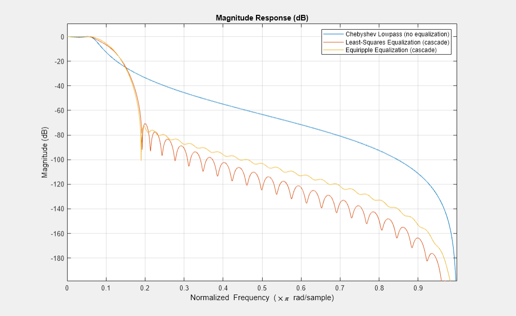
Zoom in around the passband. The passband ripples are attenuated after equalization from 0.5 dB in the original filter to 0.27 dB with the least-squares designed equalizer, and to 0.16 dB with the equiripple designed equalizer.

hfvt(2) = fvtool(Hcheby,Gls,Geq); legend(hfvt(2),'Chebyshev Lowpass (no equalization)',...'Least-Squares Equalization (cascade)',...'Equiripple Equalization (cascade)', Location ='NorthEast') hfvt(2).zoom([0 .1 -0.8 .5]);

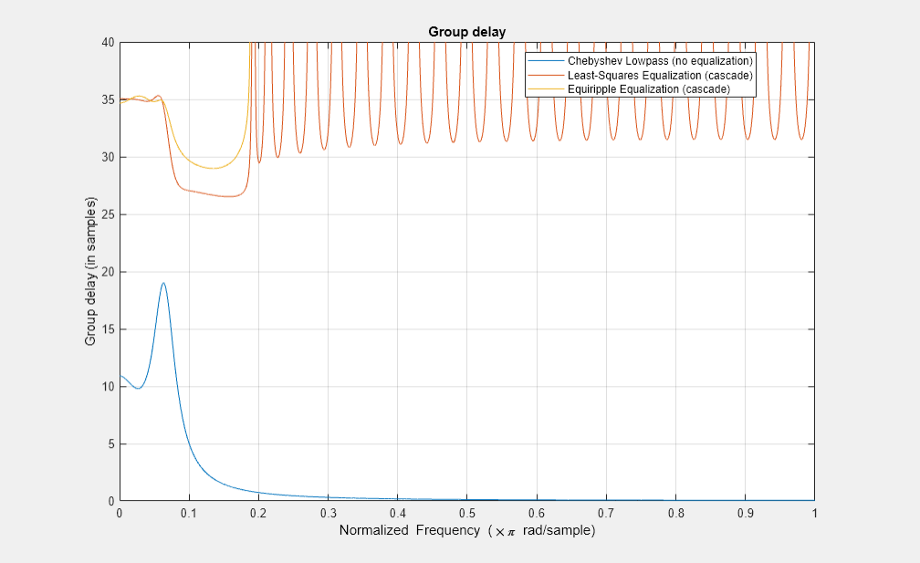
We now turn to the phase (and group delay) equalization. The combined group delay is nearly constant around 35 samples (the target group delay) on the passband. Outside the passband, the combined group delay is seemingly divergent, but this is insignificant as the gain of the filter vanishes on that region.

hfvt(2).Analysis ='grpdelay'; hfvt(2).zoom([0 1 0 40]);

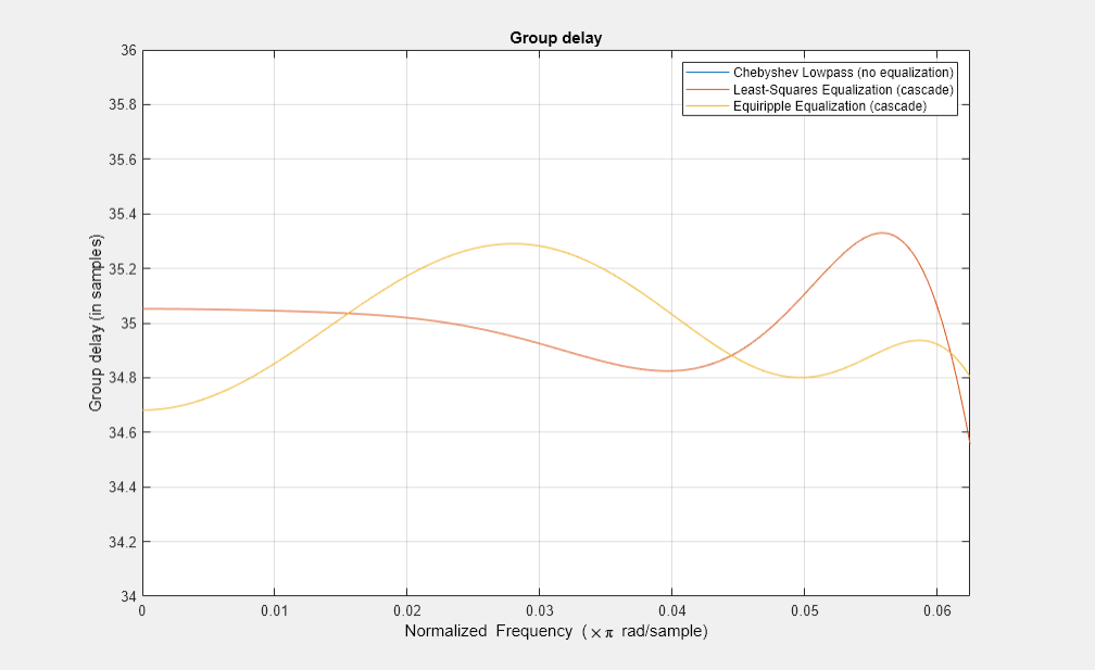
Zoom in around the passband. The group delay in the passband is equalized from a peak-to-peak difference of 8.8 samples to 0.51 samples with the least-squares equalizer, and to 0.62 samples with the equiripple equalizer. Both equalizers perform equally well.

hfvt(3) = fvtool(Hcheby,Gls,Geq,Analysis='grpdelay'); legend(hfvt(3),'Chebyshev Lowpass (no equalization)',...'Least-Squares Equalization (cascade)',...'Equiripple Equalization (cascade)', Location ='NorthEast') hfvt(3).zoom([0 Fp 34 36]);