opticalFlowFarneback
Object for estimating optical flow using Farneback method
Description
Create an optical flow object for estimating the direction and speed of moving objects using the Farneback method. Use the object functionestimateFlowto estimate the optical flow vectors. Using theresetobject function, you can reset the internal state of the optical flow object.
Creation
Description
opticFlow= opticalFlowFarneback
opticFlow= opticalFlowFarneback(Name,Value)Name,Valuepair arguments. Any unspecified properties have default values. Enclose each property name in quotes.
For example,opticalFlowFarneback('NumPyramidLevels',3)
Properties
Object Functions
estimateFlow |
Estimate optical flow |
reset |
Reset the internal state of the optical flow estimation object |
Examples
Estimate Optical Flow Using Farneback Method
Read a video file. Specify the timestamp of the frame to be read.
vidReader = VideoReader('visiontraffic.avi','CurrentTime',11);
Create an optical flow object for estimating the optical flow using Farneback method. The output is an object specifying the optical flow estimation method and its properties.
opticFlow = opticalFlowFarneback
opticFlow = opticalFlowFarneback with properties: NumPyramidLevels: 3 PyramidScale: 0.5000 NumIterations: 3 NeighborhoodSize: 5 FilterSize: 15
Create a custom figure window to visualize the optical flow vectors.
h = figure; movegui(h); hViewPanel = uipanel(h,'Position',[0 0 1 1],'Title','Plot of Optical Flow Vectors');hPlot =轴(hViewPanel);
Read the image frames and convert to grayscale images. Estimate the optical flow from consecutive image frames. Display the current image frame and plot the optical flow vectors as quiver plot.
whilehasFrame(vidReader) frameRGB = readFrame(vidReader); frameGray = rgb2gray(frameRGB); flow = estimateFlow(opticFlow,frameGray); imshow(frameRGB) holdonplot(flow,'DecimationFactor',[5 5],'ScaleFactor',2,'Parent',hPlot); holdoffpause(10^-3)end


Algorithms
The Farneback algorithm generates an image pyramid, where each level has a lower resolution compared to the previous level. When you select a pyramid level greater than 1, the algorithm can track the points at multiple levels of resolution, starting at the lowest level. Increasing the number of pyramid levels enables the algorithm to handle larger displacements of points between frames. However, the number of computations also increases. The diagram shows an image pyramid with three levels.
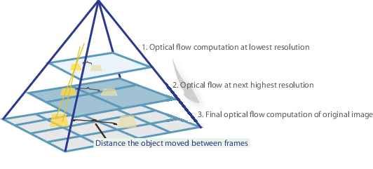
The tracking begins in the lowest resolution level, and continues until convergence. The point locations detected at a level are propagated as keypoints for the succeeding level. In this way, the algorithm refines the tracking with each level. The pyramid decomposition enables the algorithm to handle large pixel motions, which can be distances greater than the neighborhood size.
References
[1] Farneback, G. “Two-Frame Motion Estimation Based on Polynomial Expansion.” InProceedings of the 13th Scandinavian Conference on Image Analysis, 363 - 370. Halmstad, Sweden: SCIA, 2003.
Extended Capabilities
Introduced in R2015b
Select a Web Site
Choose a web site to get translated content where available and see local events and offers. Based on your location, we recommend that you select:.
Selectweb siteYou can also select a web site from the following list:
Americas
- América Latina(Español)
- Canada(English)
- United States(English)
Europe
- Belgium(English)
- Denmark(English)
- Deutschland(Deutsch)
- España(Español)
- Finland(English)
- France(Français)
- Ireland(English)
- Italia(Italiano)
- Luxembourg(English)
- Netherlands(English)
- Norway(English)
- Österreich(Deutsch)
- Portugal(English)
- Sweden(English)
- Switzerland
- United Kingdom(English)
