Discretize a Compensator

This example shows how to convert a compensator from continuous to discrete time using several discretization methods, to identify a method that yields a good match in the frequency domain.

You might design a compensator in continuous time, and then need to convert it to discrete time for a digital implementation. When you do so, you want the discretization to preserve frequency-domain characteristics that are essential to your performance and stability requirements.

In the following control system,Gis a continuous-time second-order system with a sharp resonance around 3 rad/s.

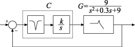
One valid controller for this system includes a notch filter in series with an integrator. Create a model of this controller.

notch = tf([1,0.5,9],[1,5,9]); integ = pid(0,0.34); C = integ*notch; bodeplot(C)

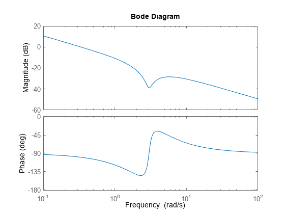
The notch filter centered at 3 rad/s counteracts the effect of the resonance inG. This configuration allows higher loop gain for a faster overall response.

Discretize the compensator.

Cdz = c2d(C,0.5);

Thec2dcommand supports several different discretization methods. Since this command does not specify a method,c2duses the default method, Zero-Order Hold (ZOH). In the ZOH method, the time-domain response of the discretized compensator matches the continuous-time response at each time step.

The discretized controllerCdz有一个示例0.5秒的时间。在实践中,sample time you choose might be constrained by the system in which you implement your controller, or by the bandwidth of your control system.

Compare the frequency-domain response ofCandCdz.

bodeplot(C,Cdz) legend('C','Cdz');

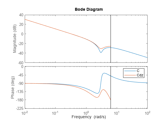
The vertical line marks the Nyquist frequency, $$\pi /T_s$$, where $$T_s$$is the sample time. Near the Nyquist frequency, the response of the discretized compensator is distorted relative to the continuous-time response. As a result, the discretized notched filter may not properly counteract the plant resonance.

To fix this, try discretizing the compensator using the Tustin method and compare to the ZOH result. The Tustin discretization method often yields a better match in the frequency domain than the ZOH method.

Cdt = c2d(C,0.5,'tustin'); plotopts = bodeoptions; plotopts.Ylim = {[-60,40],[-225,0]}; bodeplot(C,Cdz,Cdt,plotopts) legend('C','Cdz','Cdt')

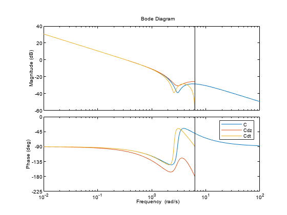
The Tustin method preserves the depth of the notch. However, the method introduces a frequency shift that is unacceptable for many applications. You can remedy the frequency shift by specifying the notch frequency as the prewarping frequency in the Tustin transform.

Discretize the compensator using the Tustin method with frequency prewarping, and compare the results.

discopts = c2dOptions('Method','tustin','PrewarpFrequency',3.0); Cdtp = c2d(C,0.5,discopts); bodeplot(C,Cdt,Cdtp,plotopts) legend('C','Cdt','Cdtp')

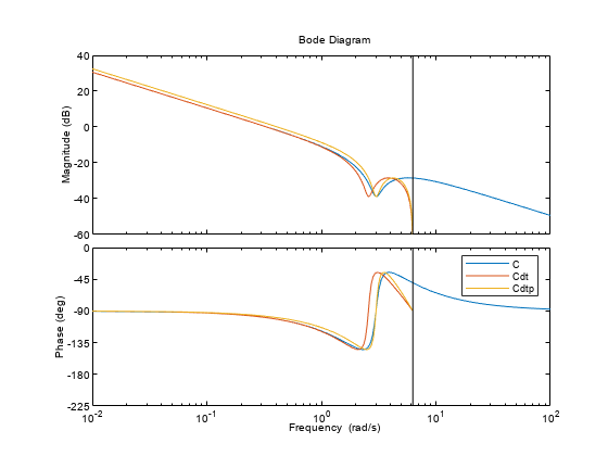
To specify additional discretization options beyond the discretization method, usec2dOptions. Here, the discretization options setdiscoptsspecifies both the Tustin method and the prewarp frequency. The prewarp frequency is 3.0 rad/s, the frequency of the notch in the compensator response.

Using the Tustin method with frequency prewarping yields a better-matching frequency response than Tustin without prewarping.

See Also

Functions

• c2d|c2dOptions

Live Editor Tasks

• Convert Model Rate

Related Topics

• Continuous-Discrete Conversion Methods
• Improve Accuracy of Discretized System with Time Delay