polyfit

Polynomial curve fitting

collapse all in page

Syntax

p = polyfit(x,y,n)

[p,S] = polyfit(x,y,n)

[p,S,mu] = polyfit(x,y,n)

Description

p= polyfit(x,y,n)returns the coefficients for a polynomialp(x)of degreenthat is a best fit (in a least-squares sense) for the data iny. The coefficients inpare in descending powers, and the length ofpisn+1

$p (x) = p_{1} x^{n} + p_{2} x^{n - 1} + ... + p_{n} x + p_{n + 1} .$

[p,S] = polyfit(x,y,n)返回一个结构Sthat can be used as an input topolyvalto obtain error estimates.

example

[p,S,mu] = polyfit(x,y,n)also returnsmu, which is a two-element vector with centering and scaling values.mu(1)ismean(x), andmu(2)isstd(x). Using these values,polyfitcentersxat zero and scales it to have unit standard deviation,

$\hat{x} = \frac{x - \bar{x}}{σ_{x}} .$

This centering and scaling transformation improves the numerical properties of both the polynomial and the fitting algorithm.

Examples

collapse all

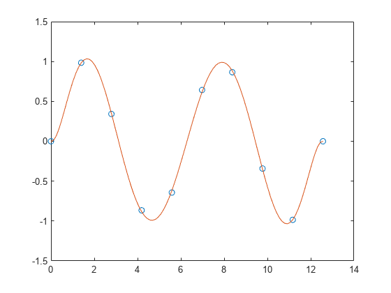
Fit Polynomial to Trigonometric Function

Open Live Script

Generate 10 points equally spaced along a sine curve in the interval[0,4*pi].

x = linspace(0,4*pi,10); y = sin(x);

Usepolyfitto fit a 7th-degree polynomial to the points.

p = polyfit(x,y,7);

Evaluate the polynomial on a finer grid and plot the results.

x1 = linspace(0,4*pi); y1 = polyval(p,x1); figure plot(x,y,'o') holdonplot(x1,y1) holdoff

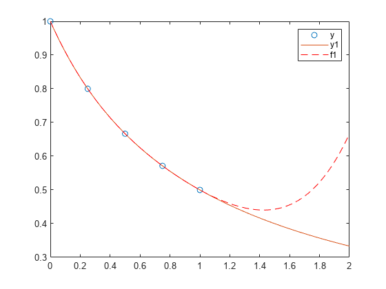
Figure contains an axes object. The axes object contains 2 objects of type line.

Fit Polynomial to Set of Points

Open Live Script

Create a vector of 5 equally spaced points in the interval[0,1], and evaluate $y (x) = (1 + x)^{- 1}$ at those points.

x = linspace(0,1,5); y = 1./(1+x);

Fit a polynomial of degree 4 to the 5 points. In general, fornpoints, you can fit a polynomial of degreen-1to exactly pass through the points.

p = polyfit(x,y,4);

Evaluate the original function and the polynomial fit on a finer grid of points between 0 and 2.

x1 = linspace(0,2); y1 = 1./(1+x1); f1 = polyval(p,x1);

Plot the function values and the polynomial fit in the wider interval[0,2], with the points used to obtain the polynomial fit highlighted as circles. The polynomial fit is good in the original[0,1]interval, but quickly diverges from the fitted function outside of that interval.

figure plot(x,y,'o') holdonplot(x1,y1) plot(x1,f1,'r--') legend('y','y1','f1')

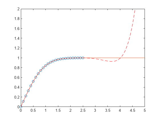
Figure contains an axes object. The axes object contains 3 objects of type line. These objects represent y, y1, f1.

Fit Polynomial to Error Function

Open Live Script

First generate a vector ofx点,等距的间隔[0,2.5], and then evaluateerf(x)at those points.

x = (0:0.1:2.5)'; y = erf(x);

Determine the coefficients of the approximating polynomial of degree 6.

p = polyfit(x,y,6)

p =1×70.0084 -0.0983 0.4217 -0.7435 0.1471 1.1064 0.0004

To see how good the fit is, evaluate the polynomial at the data points and generate a table showing the data, fit, and error.

f = polyval(p,x); T = table(x,y,f,y-f,'VariableNames',{'X','Y','Fit','FitError'})

T=26×4 tableX Y Fit FitError ___ _______ __________ ___________ 0 0 0.00044117 -0.00044117 0.1 0.11246 0.11185 0.00060836 0.2 0.2227 0.22231 0.00039189 0.3 0.32863 0.32872 -9.7429e-05 0.4 0.42839 0.4288 -0.00040661 0.5 0.5205 0.52093 -0.00042568 0.6 0.60386 0.60408 -0.00022824 0.7 0.6778 0.67775 4.6383e-05 0.8 0.7421 0.74183 0.00026992 0.9 0.79691 0.79654 0.00036515 1 0.8427 0.84238 0.0003164 1.1 0.88021 0.88005 0.00015948 1.2 0.91031 0.91035 -3.9919e-05 1.3 0.93401 0.93422 -0.000211 1.4 0.95229 0.95258 -0.00029933 1.5 0.96611 0.96639 -0.00028097 ⋮

In this interval, the interpolated values and the actual values agree fairly closely. Create a plot to show how outside this interval, the extrapolated values quickly diverge from the actual data.

x1 = (0:0.1:5)'; y1 = erf(x1); f1 = polyval(p,x1); figure plot(x,y,'o') holdonplot(x1,y1,“- - -”) plot(x1,f1,'r--') axis([0 5 0 2]) holdoff

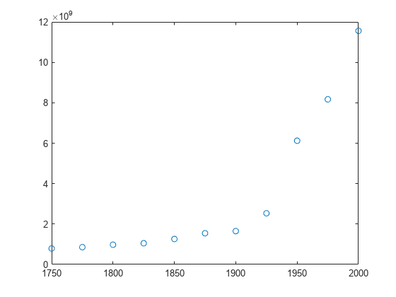
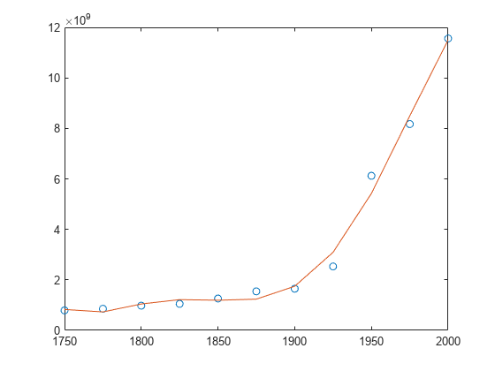
Figure contains an axes object. The axes object contains 3 objects of type line.

Use Centering and Scaling to Improve Numerical Properties

Open Live Script

Create a table of population data for the years 1750 - 2000 and plot the data points.

一年= (1750:25:2000)'; pop = 1e6*[791 856 978 1050 1262 1544 1650 2532 6122 8170 11560]'; T = table(year, pop)

T=11×2 table一年pop ____ _________ 1750 7.91e+08 1775 8.56e+08 1800 9.78e+08 1825 1.05e+09 1850 1.262e+09 1875 1.544e+09 1900 1.65e+09 1925 2.532e+09 1950 6.122e+09 1975 8.17e+09 2000 1.156e+10

plot(year,pop,'o')

Figure contains an axes object. The axes object contains an object of type line.

Usepolyfitwith three outputs to fit a 5th-degree polynomial using centering and scaling, which improves the numerical properties of the problem.polyfitcenters the data in一年at 0 and scales it to have a standard deviation of 1, which avoids an ill-conditioned Vandermonde matrix in the fit calculation.

[p,~,mu] = polyfit(T.year, T.pop, 5);

Usepolyvalwith four inputs to evaluatepwith the scaled years,(year-mu(1))/mu(2). Plot the results against the original years.

f = polyval(p,year,[],mu); holdonplot(year,f) holdoff

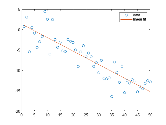
Figure contains an axes object. The axes object contains 2 objects of type line.

Simple Linear Regression

Open Live Script

Fit a simple linear regression model to a set of discrete 2-D data points.

Create a few vectors of sample data points(x,y). Fit a first degree polynomial to the data.

x = 1:50; y = -0.3*x + 2*randn(1,50); p = polyfit(x,y,1);

Evaluate the fitted polynomialpat the points inx. Plot the resulting linear regression model with the data.

f = polyval(p,x); plot(x,y,'o',x,f,“- - -”) legend('data','linear fit')

Figure contains an axes object. The axes object contains 2 objects of type line. These objects represent data, linear fit.

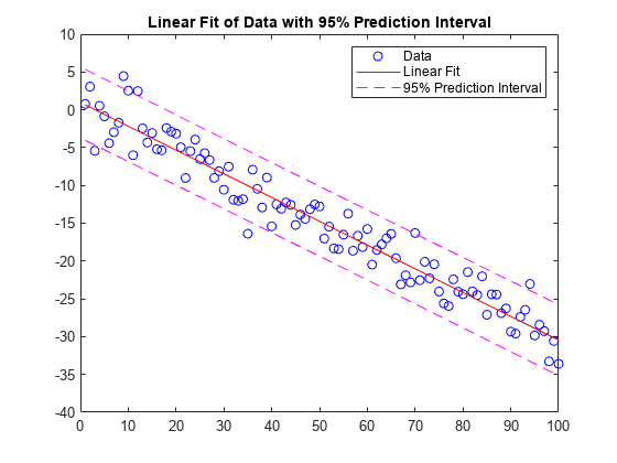
Linear Regression With Error Estimate

Open Live Script

Fit a linear model to a set of data points and plot the results, including an estimate of a 95% prediction interval.

Create a few vectors of sample data points(x,y). Usepolyfitto fit a first degree polynomial to the data. Specify two outputs to return the coefficients for the linear fit as well as the error estimation structure.

x = 1:100; y = -0.3*x + 2*randn(1,100); [p,S] = polyfit(x,y,1);

Evaluate the first-degree polynomial fit inpat the points inx. Specify the error estimation structure as the third input so thatpolyvalcalculates an estimate of the standard error. The standard error estimate is returned indelta.

[y_fit,delta] = polyval(p,x,S);

Plot the original data, linear fit, and 95% prediction interval $y \pm 2 Δ$ .

plot(x,y,'bo') holdonplot(x,y_fit,'r-') plot(x,y_fit+2*delta,'m--',x,y_fit-2*delta,'m--') title('Linear Fit of Data with 95% Prediction Interval') legend('Data','Linear Fit','95% Prediction Interval')

Figure contains an axes object. The axes object with title Linear Fit of Data with 95% Prediction Interval contains 4 objects of type line. These objects represent Data, Linear Fit, 95% Prediction Interval.

Input Arguments

collapse all

`x`—Query points
vector

Query points, specified as a vector. The points inxcorrespond to the fitted function values contained iny. Ifxis not a vector, thenpolyfitconverts it into a column vectorx(:).

Warning messages result whenxhas repeated (or nearly repeated) points or ifxmight need centering and scaling.

Data Types:single|double
Complex Number Support:Yes

`y`—Fitted values at query points
vector

Fitted values at query points, specified as a vector. The values inycorrespond to the query points contained inx. Ifyis not a vector, thenpolyfitconverts it into a column vectory(:).

Data Types:single|double
Complex Number Support:Yes

`n`—Degree of polynomial fit
positive integer scalar

Degree of polynomial fit, specified as a positive integer scalar.nspecifies the polynomial power of the left-most coefficient inp.

Output Arguments

collapse all

`p`— Least-squares fit polynomial coefficients
vector

Least-squares fit polynomial coefficients, returned as a vector.phas lengthn+1and contains the polynomial coefficients in descending powers, with the highest power beingn. If eitherxorycontainNaNvalues andn < length(x), then all elements inpareNaN.

Usepolyvalto evaluatepat query points.

`S`— Error estimation structure
structure

Error estimation structure. This optional output structure is primarily used as an input to thepolyvalfunction to obtain error estimates.Scontains the following fields:

Field	Description
`R`	Triangular`R`factor (possibly permuted) from a QR decomposition of the Vandermonde matrix of`x`
`df`	Degrees of freedom
`normr`	Norm of the residuals

If the data inyis random, then an estimate of the covariance matrix ofpis(Rinv*Rinv')*normr^2/df, whereRinvis the inverse ofR.

If the errors in the data inyare independent and normal with constant variance, then[y,delta] = polyval(...)produces error bounds that contain at least 50% of the predictions. That is,y±deltacontains at least 50% of the predictions of future observations atx.

`mu`— Centering and scaling values
two-element vector

Centering and scaling values, returned as a two-element vector.mu(1)ismean(x), andmu(2)isstd(x). These values center the query points inxat zero with unit standard deviation.

Usemuas the fourth input topolyvalto evaluatepat the scaled points,(x - mu(1))/mu(2).

Limitations

In problems with many points, increasing the degree of the polynomial fit usingpolyfitdoes not always result in a better fit. High-order polynomials can be oscillatory between the data points, leading to apoorerfit to the data. In those cases, you might use a low-order polynomial fit (which tends to be smoother between points) or a different technique, depending on the problem.
Polynomials are unbounded, oscillatory functions by nature. Therefore, they are not well-suited to extrapolating bounded data or monotonic (increasing or decreasing) data.

Algorithms

polyfitusesxto form Vandermonde matrixVwithn+1columns andm = length(x)rows, resulting in the linear system

$(\begin{matrix} x_{1}^{n} & x_{1}^{n - 1} & \dots & 1 \\ x_{2}^{n} & x_{2}^{n - 1} & \dots & 1 \\ ⋮ & ⋮ & ⋱ & ⋮ \\ x_{m}^{n} & x_{m}^{n - 1} & \dots & 1 \end{matrix}) (\begin{matrix} p_{1} \\ p_{2} \\ ⋮ \\ p_{n + 1} \end{matrix}) = (\begin{matrix} y_{1} \\ y_{2} \\ ⋮ \\ y_{m} \end{matrix}),$

whichpolyfitsolves withp = V\y. Since the columns in the Vandermonde matrix are powers of the vectorx, the condition number ofVis often large for high-order fits, resulting in a singular coefficient matrix. In those cases centering and scaling can improve the numerical properties of the system to produce a more reliable fit.

Extended Capabilities

Tall Arrays
Calculate with arrays that have more rows than fit in memory.

Usage notes and limitations:

XandY必须是列向量。

For more information, seeTall Arrays.

C/C++ Code Generation
生成C和c++代码sing MATLAB® Coder™.

Usage notes and limitations:

SeeVariable-Sizing Restrictions for Code Generation of Toolbox Functions(MATLAB Coder).

Thread-Based Environment
Run code in the background using MATLAB®`backgroundPool`or accelerate code with Parallel Computing Toolbox™`ThreadPool`.

This function fully supports thread-based environments. For more information, seeRun MATLAB Functions in Thread-Based Environment.

GPU Arrays
Accelerate code by running on a graphics processing unit (GPU) using Parallel Computing Toolbox™.

This function fully supports GPU arrays. For more information, seeRun MATLAB Functions on a GPU(Parallel Computing Toolbox).

Distributed Arrays
Partition large arrays across the combined memory of your cluster using Parallel Computing Toolbox™.

This function fully supports distributed arrays. For more information, seeRun MATLAB Functions with Distributed Arrays(Parallel Computing Toolbox).

Version History

Introduced before R2006a

polyfit

Syntax

Description

Examples

Fit Polynomial to Trigonometric Function

Fit Polynomial to Set of Points

Fit Polynomial to Error Function

Use Centering and Scaling to Improve Numerical Properties

Simple Linear Regression

Linear Regression With Error Estimate

Input Arguments

`x`—Query points
vector

`y`—Fitted values at query points
vector

`n`—Degree of polynomial fit
positive integer scalar

Output Arguments

`p`— Least-squares fit polynomial coefficients
vector

`S`— Error estimation structure
structure

`mu`— Centering and scaling values
two-element vector

Limitations

Algorithms

Extended Capabilities

Tall Arrays
Calculate with arrays that have more rows than fit in memory.

C/C++ Code Generation
生成C和c++代码sing MATLAB® Coder™.

Thread-Based Environment
Run code in the background using MATLAB®`backgroundPool`or accelerate code with Parallel Computing Toolbox™`ThreadPool`.

GPU Arrays
Accelerate code by running on a graphics processing unit (GPU) using Parallel Computing Toolbox™.

Distributed Arrays
Partition large arrays across the combined memory of your cluster using Parallel Computing Toolbox™.

Version History

See Also

Topics

polyfit

Syntax

Description

Examples

Fit Polynomial to Trigonometric Function

Fit Polynomial to Set of Points

Fit Polynomial to Error Function

Use Centering and Scaling to Improve Numerical Properties

Simple Linear Regression

Linear Regression With Error Estimate

Input Arguments

x—Query pointsvector

y—Fitted values at query pointsvector

n—Degree of polynomial fitpositive integer scalar

Output Arguments

p— Least-squares fit polynomial coefficientsvector

S— Error estimation structurestructure

mu— Centering and scaling valuestwo-element vector

Limitations

Algorithms

Extended Capabilities

Tall ArraysCalculate with arrays that have more rows than fit in memory.

C/C++ Code Generation生成C和c++代码sing MATLAB® Coder™.

Thread-Based EnvironmentRun code in the background using MATLAB®backgroundPoolor accelerate code with Parallel Computing Toolbox™ThreadPool.

GPU ArraysAccelerate code by running on a graphics processing unit (GPU) using Parallel Computing Toolbox™.

Distributed ArraysPartition large arrays across the combined memory of your cluster using Parallel Computing Toolbox™.

Version History

See Also

Topics

`x`—Query points
vector

`y`—Fitted values at query points
vector

`n`—Degree of polynomial fit
positive integer scalar

`p`— Least-squares fit polynomial coefficients
vector

`S`— Error estimation structure
structure

`mu`— Centering and scaling values
two-element vector

Tall Arrays
Calculate with arrays that have more rows than fit in memory.

C/C++ Code Generation
生成C和c++代码sing MATLAB® Coder™.

Thread-Based Environment
Run code in the background using MATLAB®`backgroundPool`or accelerate code with Parallel Computing Toolbox™`ThreadPool`.

GPU Arrays
Accelerate code by running on a graphics processing unit (GPU) using Parallel Computing Toolbox™.

Distributed Arrays
Partition large arrays across the combined memory of your cluster using Parallel Computing Toolbox™.