Compare Robust Regression Techniques

Open Live Script

This example compares the results among regression techniques that are and are not robust to influential outliers.

Influential outliersare extreme response or predictor observations that influence parameter estimates and inferences of a regression analysis. Responses that are influential outliers typically occur at the extremes of a domain. For example, you might have an instrument that measures a response poorly or erratically at extreme levels of temperature.

With enough evidence, you can remove influential outliers from the data. If removal is not possible, you can use regression techniques that are robust to outliers.

Simulate Data

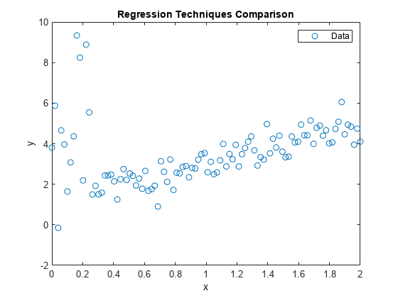
Generate a random sample of 100 responses from the linear model

$y_{t} = 1 + 2 x_{t} + ε_{t}$

where:

$x$ is a vector of evenly spaced values from 0 through 2.
$ε_{t} \sim N (0, 0 ． 5^{2}) ．$

rng('default');n = 100;x = linspace (0 2 n) ';b0 = 1;b1 = 2;sigma = 0.5; e = randn(n,1); y = b0 + b1*x + sigma*e;

Create influential outliers by inflating all responses corresponding to $x < 0 ． 25$ by a factor of 3.

y(x < 0.25) = y(x < 0.25)*3;

Plot the data. Retain the plot for further graphs.

figure; plot(x,y,'o');h = gca; xlim = h.XLim'; hl = legend('Data');xlabel('x');ylabel('y');title('Regression Techniques Comparison') holdon;

Figure contains an axes object. The axes object with title Regression Techniques Comparison contains an object of type line. This object represents Data.

Estimate Linear Model

我们估计系数和误差方差ing simple linear regression. Plot the regression line.

LSMdl = fitlm(x,y)

LSMdl = Linear regression model: y ~ 1 + x1 Estimated Coefficients: Estimate SE tStat pValue ________ _______ ______ __________ (Intercept) 2.6814 0.28433 9.4304 2.0859e-15 x1 0.78974 0.24562 3.2153 0.0017653 Number of observations: 100, Error degrees of freedom: 98 Root Mean Squared Error: 1.43 R-squared: 0.0954, Adjusted R-Squared: 0.0862 F-statistic vs. constant model: 10.3, p-value = 0.00177

plot(xlim,[ones(2,1) xlim]*LSMdl.Coefficients.Estimate,'LineWidth',2); hl.String{2} ='Least Squares';

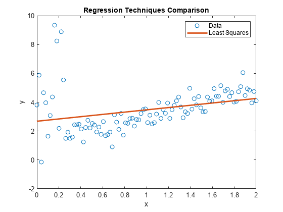
Figure contains an axes object. The axes object with title Regression Techniques Comparison contains 2 objects of type line. These objects represent Data, Least Squares.

LSMdlis a fittedLinearModelmodel object. The intercept and slope appear to be respectively higher and lower than they should be. The regression line might make poor predictions for any $x < 1$ and $x > 1 ． 6$ ．

Estimate Bayesian Linear Regression Model with Diffuse Prior Distribution

Create a Bayesian linear regression model with a diffuse joint prior for the regression coefficients and error variance. Specify one predictor for the model.

PriorDiffuseMdl = bayeslm(1);

PriorDiffuseMdlis adiffuseblmmodel object that characterizes the joint prior distribution.

Estimate the posterior of the Bayesian linear regression model. Plot the regression line.

PosteriorDiffuseMdl = estimate(PriorDiffuseMdl,x,y);

Method: Analytic posterior distributions Number of observations: 100 Number of predictors: 2 | Mean Std CI95 Positive Distribution ------------------------------------------------------------------------------ Intercept | 2.6814 0.2873 [ 2.117, 3.246] 1.000 t (2.68, 0.28^2, 98) Beta | 0.7897 0.2482 [ 0.302, 1.277] 0.999 t (0.79, 0.25^2, 98) Sigma2 | 2.0943 0.3055 [ 1.580, 2.773] 1.000 IG(49.00, 0.0099)

plot(xlim,[ones(2,1) xlim]*PosteriorDiffuseMdl.Mu,'--','LineWidth',2); hl.String{3} ='Bayesian Diffuse';

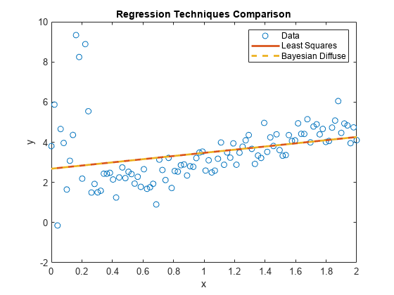
Figure contains an axes object. The axes object with title Regression Techniques Comparison contains 3 objects of type line. These objects represent Data, Least Squares, Bayesian Diffuse.

PosteriorDiffuseMdlis aconjugateblmmodel object that characterizes the joint posterior distribution of the linear model parameters. The estimates of a Bayesian linear regression model with diffuse prior are almost equal to those of a simple linear regression model. Both models represent a naive approach to influential outliers, that is, the techniques treat outliers like any other observation.

Estimate Regression Model with ARIMA Errors

Create a regression model with ARIMA errors. Specify that the errors follow atdistribution with 3 degrees of freedom, but no lagged terms. This specification is effectively a regression model withtdistributed errors.

regMdl = regARIMA(0,0,0); regMdl.Distribution = struct('Name','t','DoF',3);

regMdlis aregARIMAmodel object. It is a template for estimation.

Estimate the regression model with ARIMA errors. Plot the regression line.

estRegMdl = estimate(regMdl,y,'X',x);

Regression with ARMA(0,0) Error Model (t Distribution): Value StandardError TStatistic PValue _______ _____________ __________ __________ Intercept 1.4613 0.154 9.4892 2.328e-21 Beta(1) 1.6531 0.12939 12.776 2.2246e-37 Variance 0.93116 0.1716 5.4263 5.7546e-08 DoF 3 0 Inf 0

plot(xlim,[ones(2,1) xlim]*[estRegMdl.Intercept; estRegMdl.Beta],．..'LineWidth',2); hl.String{4} ='regARIMA';

Figure contains an axes object. The axes object with title Regression Techniques Comparison contains 4 objects of type line. These objects represent Data, Least Squares, Bayesian Diffuse, regARIMA.

estRegMdlis aregARIMAmodel object containing the estimation results. Because thetdistribution is more diffuse, the regression line attributes more variability to the influential outliers than to the other observations. Therefore, the regression line appears to be a better predictive model than the other models.

Implement Quantile Regression Using Bag of Regression Trees

Grow a bag of 100 regression trees. Specify 20 for the minimum leaf size.

QRMdl = TreeBagger(100,x,y,'Method','regression','MinLeafSize',20);

QRMdlis a fittedTreeBaggermodel object.

Predict median responses for all observed $x$ values, that is, implement quantile regression. Plot the predictions.

qrPred = quantilePredict(QRMdl,x); plot(x,qrPred,'LineWidth',2); hl.String{5} ='Quantile'; holdoff;

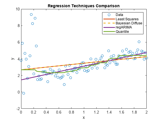
Figure contains an axes object. The axes object with title Regression Techniques Comparison contains 5 objects of type line. These objects represent Data, Least Squares, Bayesian Diffuse, regARIMA, Quantile.

The regression line appears to be slightly influenced by the outliers at the beginning of the sample, but then quickly follows theregARIMAmodel line.

You can adjust the behavior of the line by specifying various values forMinLeafSizewhen you train the bag of regression trees. LowerMinLeafSizevalues tend to follow the data in the plot more closely.

Implement Robust Bayesian Linear Regression

Consider a Bayesian linear regression model containing a one predictor, at分布式disturbance variance with a profiled degrees of freedom parameter $ν$ ．Let:

$λ_{j} \sim I G (ν / 2, 2 / ν)$ ．
$ε_{j} | λ_{j} \sim N (0, λ_{j} σ^{2})$
$f (β, σ^{2}) \propto \frac{1}{σ^{2}}$

These assumptions imply:

$ε_{j} \sim t (0, σ^{2}, ν)$
$λ_{j} | ε_{j} \sim I G (\frac{ν + 1}{2}, \frac{2}{ν + ε_{j}^{2} / σ^{2}})$

$λ$ is a vector of latent scale parameters that attributes low precision to observations that are far from the regression line. $ν$ is a hyperparameter controlling the influence of $λ$ on the observations.

Specify a grid of values for $ν$ ．

1corresponds to the Cauchy distribution.
2.1means that the mean is well-defined.
4.1 means that the variance is well-defined.
100means that the distribution is approximately normal.

nu = [0.01 0.1 1 2.1 5 10 100]; numNu = numel(nu);

For this problem, the Gibbs sampler is well-suited to estimate the coefficients because you can simulate the parameters of a Bayesian linear regression model conditioned on $λ$ , and then simulate $λ$ from its conditional distribution.

Implement this Gibbs sampler.

Draw parameters from the posterior distribution of $β, σ^{2} | y, x, λ$ ．缩小的观察 $λ$ , create a diffuse prior model with two regression coefficients, and draw a set of parameters from the posterior. The first regression coefficient corresponds to the intercept, so specify thatbayeslmnot include one.
Compute residuals.
Draw values from the conditional posterior of $λ$ ．

For each value of $ν$ , run the Gibbs sampler for 20,000 iterations and apply a burn-in period of 5,000. Preallocate for the posterior draws and initialize $λ$ to a vector of ones.

rng(1); m = 20000; burnin = 5000; lambda = ones(n,m + 1,numNu);% PreallocationestBeta = zeros(2,m + 1,numNu); estSigma2 = zeros(1,m + 1,numNu);% Create diffuse prior model.PriorMdl = bayeslm(2,'Model','diffuse','Intercept',false);forp = 1:numNuforj = 1:m% Scale observations.yDef = y./sqrt(lambda(:,j,p)); xDef = [ones(n,1) x]./sqrt(lambda(:,j,p));% Simulate observations from conditional posterior of beta and% sigma2 given lambda and the data.[estBeta(:,j + 1,p),estSigma2(1,j + 1,p)] = simulate(PriorMdl,xDef,yDef);% Estimate residuals.ep = y - [ones(n,1) x]*estBeta(:,j + 1,p);% Specify shape and scale using conditional posterior of lambda% given beta, sigma2, and the datasp = (nu(p) + 1)/2; sc = 2./(nu(p) + ep.^2/estSigma2(1,j + 1,p));% Draw from conditional posterior of lambda given beta, sigma2,% and the datalambda(:,j + 1,p) = 1./gamrnd(sp,sc);endend

Estimate posterior means for $β$ , $σ^{2}$ , and $λ$ ．

postEstBeta = squeeze(mean(estBeta(:,(burnin+1):end,:),2)); postLambda = squeeze(mean(lambda(:,(burnin+1):end,:),2));

For each $ν$ , plot the data and regression lines.

figure; plot(x,y,'o');h = gca; xlim = h.XLim'; ylim = h.YLim; hl = legend('Data');holdon;forp = 1:numNu; plotY = [ones(2,1) xlim]*postEstBeta(:,p); plot(xlim,plotY,'LineWidth',2); hl.String{p+1} = sprintf('nu = %f',nu(p));endxlabel('x');ylabel('y');title('Robust Bayesian Linear Regression')

Figure contains an axes object. The axes object with title Robust Bayesian Linear Regression contains 8 objects of type line. These objects represent Data, nu = 0.010000, nu = 0.100000, nu = 1.000000, nu = 2.100000, nu = 5.000000, nu = 10.000000, nu = 100.000000.

Low values of $ν$ tend to attribute high variability to the influential outliers. Therefore, the regression line resembles theregARIMAline. As $ν$ increases, the line behaves more like those of the naive approach.

Compare Robust Regression Techniques

Simulate Data

Estimate Linear Model

Estimate Bayesian Linear Regression Model with Diffuse Prior Distribution

Estimate Regression Model with ARIMA Errors

Implement Quantile Regression Using Bag of Regression Trees

Implement Robust Bayesian Linear Regression

See Also

Functions

Objects

Related Topics

Econometrics Toolbox Documentation

万博1manbetx

A Practical Guide to Modeling Financial Risk with MATLAB