Robust Controller for Spinning Satellite

Plant model

The plant model is the same as described inMIMO Stability Margins for Spinning Satellite.

a = 10; A = [0 a;-a 0]; B = eye(2); C = [1 a;-a 1]; D = 0; Gnom = ss(A,B,C,D);

Nominal Mixed-Sensitivity Design

Start with a basic mixed-sensitivity design usingmixsyn. Pick the weights to achieve good performance while limiting bandwidth and control effort. (SeeMixed-Sensitivity Loop Shapingfor details about this technique and how to choose weighting functions.)

wS = makeweight(1e3,1,1e-1); wKS = makeweight(0.5,[500 1e2],1e4,0,2); wT = makeweight(0.5,20,100); bodemag(wS,wKS,wT), grid legend('wS','wKS','wT')

Compute the optimal MIMO controllerK1withmixsyn.

[K1,~,gam] = mixsyn(Gnom,wS,wKS,wT); gam

gam = 0.7166

The optimal performance is about 0.7, indicating thatmixsyneasily met the bounds on $$S,KS,T$$. Close the feedback loop and plot the step response.

T = feedback(Gnom*K1,eye(2)); step(T,2), grid

The nominal responses are fast with little overshoot.

Disk Margins

To gauge the robustness of this controller, check the disk margins at the plant inputs and the plant outputs.

diskmarginplot(K1*Gnom,'b',Gnom*K1,'r--') grid legend('At plant inputs','At plant outputs')

Both are good with near 10 dB gain margin and 50 degrees phase margin. Also check the disk margins when the gain and phase are allowed to vary at both the inputs and outputs of the plant.

MMIO = diskmargin(Gnom,K1)

MMIO =struct with fields:GainMargin: [0.9915 1.0085] PhaseMargin: [-0.4863 0.4863] DiskMargin: 0.0085 LowerBound: 0.0085 UpperBound: 0.0085 Frequency: 9.9988 WorstPerturbation: [1x1 struct]

The I/O margins are extremely small. This first design also lacks robustness. You can confirm the poor robustness by injecting the smallest destabilizing perturbations returned bydiskmarginat the plant inputs and outputs. (Seediskmarginfor further details about theWorstPerturbationfield of its output structures.)

WP = MMIO.WorstPerturbation; bode(WP.Input,WP.Output) title('Smallest destabilizing perturbation') legend('Input perturbation','Output perturbation')

Tpert = feedback(WP.Output*Gnom*WP.Input*K1,eye(2)); step(Tpert,5) grid

The step response continues to oscillate after the initial transient indicating marginal instability. Verify that the perturbed closed-loop systemTperthas a pole on the imaginary axis at the critical frequencyMMIO.Frequency.

[wn,zeta] = damp(Tpert); [~,idx] = min(zeta); [zeta(idx) wn(idx) MMIO.Frequency]

ans =1×30.0000 9.9988 9.9988

Robust Design

Create an uncertain plant model where the parametera(spinning frequency) varies in the range [7 13].

a = ureal('a',10,'range',[7 13]); A = [0 a;-a 0]; B = eye(2); C = [1 a;-a 1]; D = 0; Gunc = ss(A,B,C,D);

You can usemusynto design a robust controller for this uncertain plant. To improve robustness, use theumargin元素在bot模式增益和相位的不确定性h inputs and outputs, so that musyn enforces robustness for the modeled range of uncertainty. Suppose that you want at least 2 dB gain margin at each I/O (4 dB total for each channel). If yourumarginelements model that full range of variation,musynmight not yield good results, because it attempts to enforce robust performance over the modeled uncertainty as well as robust stability.musynmost likely cannot maintained the desired performance for that much gain variation. Instead, scale back the target to 1 dB gain variation in each I/O.

GM = 1.1;% about 1 dBu1 = umargin('u1',GM); u2 = umargin('u2',GM); y1 = umargin('y1',GM); y2 = umargin('y2',GM); InputMargins = append(u1,u2); OutputMargins = append(y1,y2); Gunc = OutputMargins*Gunc*InputMargins;

Augment the plant with the mixed-sensitivity weights and usemusynto optimize robust performance for the modeled uncertainty, which includes both the parameteraand the gain and phase variations at plant inputs and outputs.

P = augw(Gunc,wS,wKS,wT); [K2,gam] = musyn(P,2,2);

D-K ITERATION SUMMARY: ----------------------------------------------------------------- Robust performance Fit order ----------------------------------------------------------------- Iter K Step Peak MU D Fit D 1 175.9 2.593 2.606 24 2 1.21 1.21 1.223 56 3 1.167 1.167 1.183 64 4 1.168 1.168 1.199 52 5 1.201 1.2 1.201 58 Best achieved robust performance: 1.17

强劲的性能is close to 1, indicating that the controller is close to robustly meeting the mixed-sensitivity goals. Check the disk margins at the plant I/Os.

MMIO = diskmargin(Gnom,K2)

MMIO =struct with fields:GainMargin: [0.6406 1.5610] PhaseMargin: [-24.7101 24.7101] DiskMargin: 0.4381 LowerBound: 0.4381 UpperBound: 0.4459 Frequency: 2.7917 WorstPerturbation: [1x1 struct]

The margins are now about 1.6 dB and 25 degrees, much better than before. Compare the step responses with each controller for 25 uncertainty samples.

T1 = feedback(Gunc*K1,eye(2)); T2 = feedback(Gunc*K2,eye(2)); rng(0)% for reproducibilityT1s = usample(T1,25); rng(0) T2s = usample(T2,25); opt = timeoptions; opt.YLim = {[-1 1.5]}; stepplot(T1s,T2s,4,opt) grid legend('Nominal design','Robust design','location','southeast')

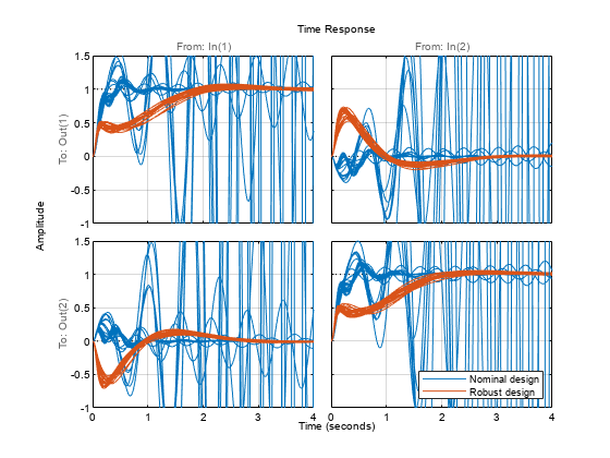
The second design is a clear improvement. Further compare the sensitivity and complementary sensitivity functions.

sigma(eye(2)-T1s,eye(2)-T2s), grid axis([1e-2 1e4 -80 20]) title('Sensitivity') legend('Nominal design','Robust design','location','southeast')

sigma(T1s,T2s), grid axis([1e-2 1e4 -80 20]) title(“互补敏感性”) legend('Nominal design','Robust design','location','southeast')

This example has shown how to use theumarginuncertain element to improve stability margins as part of a robust controller synthesis.