Main Content

resubLoss

Resubstitution classification loss for naive Bayes classifier

Description

example

L= resubLoss(Mdl)returns theClassification Lossby resubstitution (L) or the in-sample classification loss, for the naive Bayes classifierMdlusing the training data stored inMdl.Xand the corresponding class labels stored inMdl.Y.

The classification loss (L) is a generalization or resubstitution quality measure. Its interpretation depends on the loss function and weighting scheme; in general, better classifiers yield smaller classification loss values.

example

L= resubLoss(Mdl,'LossFun',LossFun)returns the classification loss by resubstitution using the loss function supplied inLossFun.

Examples

collapse all

Determine the in-sample classification error (resubstitution loss) of a naive Bayes classifier. In general, a smaller loss indicates a better classifier.

Load thefisheririsdata set. CreateXas a numeric matrix that contains four petal measurements for 150 irises. CreateYas a cell array of character vectors that contains the corresponding iris species.

loadfisheririsX = meas; Y = species;

Train a naive Bayes classifier using the predictorsXand class labelsY. A recommended practice is to specify the class names.fitcnbassumes that each predictor is conditionally and normally distributed.

Mdl = fitcnb(X,Y,'ClassNames',{'setosa','versicolor','virginica'})
Mdl = ClassificationNaiveBayes ResponseName:‘Y’CategoricalPredictors: [] ClassNames: {'setosa' 'versicolor' 'virginica'} ScoreTransform: 'none' NumObservations: 150 DistributionNames: {'normal' 'normal' 'normal' 'normal'} DistributionParameters: {3x4 cell} Properties, Methods

Mdlis a trainedClassificationNaiveBayesclassifier.

Estimate the in-sample classification error.

L = resubLoss(Mdl)
L = 0.0400

The naive Bayes classifier misclassifies 4% of the training observations.

Load thefisheririsdata set. CreateXas a numeric matrix that contains four petal measurements for 150 irises. CreateYas a cell array of character vectors that contains the corresponding iris species.

loadfisheririsX = meas; Y = species;

Train a naive Bayes classifier using the predictorsXand class labelsY. A recommended practice is to specify the class names.fitcnbassumes that each predictor is conditionally and normally distributed.

Mdl = fitcnb(X,Y,'ClassNames',{'setosa','versicolor','virginica'});

Mdlis a trainedClassificationNaiveBayesclassifier.

Estimate the logit resubstitution loss.

L = resubLoss(Mdl,'LossFun','logit')
L = 0.3310

The average in-sample logit loss is approximately 0.33.

Input Arguments

collapse all

Full, trained naive Bayes classifier, specified as aClassificationNaiveBayesmodel trained byfitcnb.

Loss function, specified as a built-in loss function name or function handle.

  • The following table lists the available loss functions. Specify one using its corresponding character vector or string scalar.

    Value Description
    'binodeviance' Binomial deviance
    'classiferror' Classification error
    'exponential' Exponential
    'hinge' Hinge
    'logit' Logistic
    'mincost' Minimal expected misclassification cost (for classification scores that are posterior probabilities)
    'quadratic' Quadratic

    'mincost'is appropriate for classification scores that are posterior probabilities. Naive Bayes models return posterior probabilities as classification scores by default (seepredict).

  • Specify your own function using function handle notation.

    Suppose thatnis the number of observations inXandKis the number of distinct classes (numel(Mdl.ClassNames), whereMdlis the input model). Your function must have this signature

    lossvalue =lossfun(C,S,W,Cost)
    where:

    • The output argumentlossvalueis a scalar.

    • You specify the function name (lossfun).

    • Cis ann-by-Klogical matrix with rows indicating the class to which the corresponding observation belongs. The column order corresponds to the class order inMdl.ClassNames.

      CreateCby settingC(p,q) = 1如果观察pis in classq,为每一行。设置所有其他元素的行pto0.

    • Sis ann-by-Knumeric matrix of classification scores. The column order corresponds to the class order inMdl.ClassNames.Sis a matrix of classification scores, similar to the output ofpredict.

    • Wis ann-by-1 numeric vector of observation weights. If you passW, the software normalizes the weights to sum to1.

    • Costis aK-by-Knumeric matrix of misclassification costs. For example,Cost = ones(K) - eye(K)specifies a cost of0for correct classification and1for misclassification.

    Specify your function using'LossFun',@lossfun.

For more details on loss functions, seeClassification Loss.

Data Types:char|string|function_handle

More About

collapse all

Classification Loss

Classification lossfunctions measure the predictive inaccuracy of classification models. When you compare the same type of loss among many models, a lower loss indicates a better predictive model.

Consider the following scenario.

  • Lis the weighted average classification loss.

  • nis the sample size.

  • For binary classification:

    • yjis the observed class label. The software codes it as –1 or 1, indicating the negative or positive class, respectively.

    • f(Xj) is the raw classification score for observation (row)jof the predictor dataX.

    • mj=yjf(Xj) is the classification score for classifying observationjinto the class corresponding toyj. Positive values ofmjindicate correct classification and do not contribute much to the average loss. Negative values ofmjindicate incorrect classification and contribute significantly to the average loss.

  • For algorithms that support multiclass classification (that is,K≥ 3):

    • yj*is a vector ofK– 1 zeros, with 1 in the position corresponding to the true, observed classyj. For example, if the true class of the second observation is the third class andK= 4, theny2*= [0 0 1 0]′. The order of the classes corresponds to the order in theClassNamesproperty of the input model.

    • f(Xj) is the lengthKvector of class scores for observationjof the predictor dataX. The order of the scores corresponds to the order of the classes in theClassNamesproperty of the input model.

    • mj=yj*f(Xj). Therefore,mjis the scalar classification score that the model predicts for the true, observed class.

  • The weight for observationjiswj. The software normalizes the observation weights so that they sum to the corresponding prior class probability. The software also normalizes the prior probabilities so they sum to 1. Therefore,

    j = 1 n w j = 1.

Given this scenario, the following table describes the supported loss functions that you can specify by using the'LossFun'name-value pair argument.

Loss Function Value ofLossFun Equation
Binomial deviance 'binodeviance' L = j = 1 n w j log { 1 + exp [ 2 m j ] } .
Exponential loss 'exponential' L = j = 1 n w j exp ( m j ) .
Classification error 'classiferror'

L = j = 1 n w j I { y ^ j y j } .

The classification error is the weighted fraction of misclassified observations where y ^ j is the class label corresponding to the class with the maximal posterior probability.I{x} is the indicator function.

Hinge loss 'hinge' L = j = 1 n w j max { 0 , 1 m j } .
Logit loss 'logit' L = j = 1 n w j log ( 1 + exp ( m j ) ) .
Minimal cost 'mincost'

The software computes the weighted minimal cost using this procedure for observationsj= 1,...,n.

  1. Estimate the 1-by-Kvector of expected classification costs for observationj:

    γ j = f ( X j ) C .

    f(Xj) is the column vector of class posterior probabilities for binary and multiclass classification.Cis the cost matrix stored by the input model in theCostproperty.

  2. For observationj, predict the class label corresponding to the minimum expected classification cost:

    y ^ j = min j = 1 , ... , K ( γ j ) .

  3. UsingC, identify the cost incurred (cj) for making the prediction.

The weighted, average, minimum cost loss is

L = j = 1 n w j c j .

Quadratic loss 'quadratic' L = j = 1 n w j ( 1 m j ) 2 .

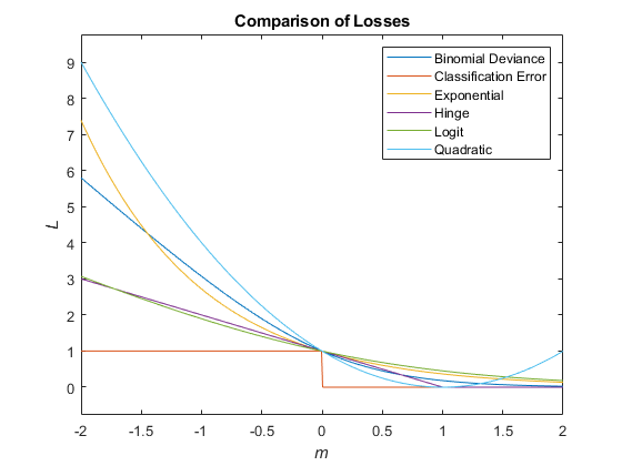
This figure compares the loss functions (except'mincost') for one observation overm. Some functions are normalized to pass through [0,1].

Comparison of classification losses for different loss functions

Posterior Probability

Theposterior probabilityis the probability that an observation belongs in a particular class, given the data.

For naive Bayes, the posterior probability that a classification iskfor a given observation (x1,...,xP) is

P ^ ( Y = k | x 1 , .. , x P ) = P ( X 1 , ... , X P | y = k ) π ( Y = k ) P ( X 1 , ... , X P ) ,

where:

  • P ( X 1 , ... , X P | y = k ) is the conditional joint density of the predictors given they are in classk.Mdl.DistributionNamesstores the distribution names of the predictors.

  • π(Y=k) is the class prior probability distribution.Mdl.Priorstores the prior distribution.

  • P ( X 1 , .. , X P ) is the joint density of the predictors. The classes are discrete, so P ( X 1 , ... , X P ) = k = 1 K P ( X 1 , ... , X P | y = k ) π ( Y = k ) .

Prior Probability

Theprior probabilityof a class is the assumed relative frequency with which observations from that class occur in a population.

Introduced in R2014b