Build a Map from Lidar Data
This example shows how to process 3-D lidar data from a sensor mounted on a vehicle to progressively build a map, with assistance from inertial measurement unit (IMU) readings. Such a map can facilitate path planning for vehicle navigation or can be used for localization. For evaluating the generated map, this example also shows how to compare the trajectory of the vehicle against global positioning system (GPS) recording.
Overview
High Definition (HD) maps are mapping services that provide precise geometry of roads up to a few centimeters in accuracy. This level of accuracy makes HD maps suitable for automated driving workflows such as localization and navigation. Such HD maps are generated by building a map from 3-D lidar scans, in conjunction with high-precision GPS and or IMU sensors and can be used to localize a vehicle within a few centimeters. This example implements a subset of features required to build such a system.
In this example, you learn how to:
Load, explore and visualize recorded driving data
Build a map using lidar scans
Improve the map using IMU readings
Load and Explore Recorded Driving Data
The data used in this example is fromthis GitHub® repository, and represents approximately 100 seconds of lidar, GPS and IMU data. The data is saved in the form of MAT-files, each containing atimetable. Download the MAT-files from the repository and load them into the MATLAB® workspace.
Note:This download can take a few minutes.
baseDownloadURL =“https://github.com/mathworks/udacity-self-driving-data-subset/raw/master/drive_segment_11_18_16/'; dataFolder = fullfile(tempdir,'drive_segment_11_18_16', filesep); options = weboptions('Timeout', Inf); lidarFileName = dataFolder +"lidarPointClouds.mat"; imuFileName = dataFolder +"imuOrientations.mat"; gpsFileName = dataFolder +"gpsSequence.mat"; folderExists = exist(dataFolder,'dir'); matfilesExist = exist(lidarFileName,'file') && exist(imuFileName,'file')...&& exist(gpsFileName,'file');if~folderExists mkdir(dataFolder);endif~ matfilesExist disp ('Downloading lidarPointClouds.mat (613 MB)...') websave(lidarFileName, baseDownloadURL +"lidarPointClouds.mat", options); disp('Downloading imuOrientations.mat (1.2 MB)...') websave(imuFileName, baseDownloadURL +"imuOrientations.mat", options); disp('Downloading gpsSequence.mat (3 KB)...') websave (gpsFileName baseDownloadURL +"gpsSequence.mat", options);end
First, load the point cloud data saved from a Velodyne® HDL32E lidar. Each scan of lidar data is stored as a 3-D point cloud using thepointCloudobject. This object internally organizes the data using a K-d tree data structure for faster search. The timestamp associated with each lidar scan is recorded in theTimevariable of the timetable.
% Load lidar data from MAT-filedata = load(lidarFileName); lidarPointClouds = data.lidarPointClouds;% Display first few rows of lidar datahead(lidarPointClouds)
Time PointCloud _____________ ______________ 23:46:10.5115 1×1 pointCloud 23:46:10.6115 1×1 pointCloud 23:46:10.7116 1×1 pointCloud 23:46:10.8117 1×1 pointCloud 23:46:10.9118 1×1 pointCloud 23:46:11.0119 1×1 pointCloud 23:46:11.1120 1×1 pointCloud 23:46:11.2120 1×1 pointCloud
Load the GPS data from the MAT-file. TheLatitude,Longitude, andAltitudevariables of thetimetableare used to store the geographic coordinates recorded by the GPS device on the vehicle.
% Load GPS sequence from MAT-filedata = load(gpsFileName); gpsSequence = data.gpsSequence;% Display first few rows of GPS datahead(gpsSequence)
Time Latitude Longitude Altitude _____________ ________ _________ ________ 23:46:11.4563 37.4 -122.11 -42.5 23:46:12.4563 37.4 -122.11 -42.5 23:46:13.4565 37.4 -122.11 -42.5 23:46:14.4455 37.4 -122.11 -42.5 23:46:15.4455 37.4 -122.11 -42.5 23:46:16.4567 37.4 -122.11 -42.5 23:46:17.4573 37.4 -122.11 -42.5 23:46:18.4656 37.4 -122.11 -42.5
加载MAT-file IMU数据。一个IMU迪比卡lly consists of individual sensors that report information about the motion of the vehicle. They combine multiple sensors, including accelerometers, gyroscopes and magnetometers. TheOrientationvariable stores the reported orientation of the IMU sensor. These readings are reported as quaternions. Each reading is specified as a 1-by-4 vector containing the four quaternion parts. Convert the 1-by-4 vector to aquaternion(Automated Driving Toolbox)object.
% Load IMU recordings from MAT-filedata = load(imuFileName); imuOrientations = data.imuOrientations;% Convert IMU recordings to quaternion typeimuOrientations = convertvars(imuOrientations,'Orientation','quaternion');% Display first few rows of IMU datahead(imuOrientations)
Time Orientation _____________ ______________ 23:46:11.4570 1×1 quaternion 23:46:11.4605 1×1 quaternion 23:46:11.4620 1×1 quaternion 23:46:11.4655 1×1 quaternion 23:46:11.4670 1×1 quaternion 23:46:11.4705 1×1 quaternion 23:46:11.4720 1×1 quaternion 23:46:11.4755 1×1 quaternion
To understand how the sensor readings come in, for each sensor, compute the approximate frameduration.
lidarFrameDuration = median(diff(lidarPointClouds.Time)); gpsFrameDuration = median(diff(gpsSequence.Time)); imuFrameDuration = median(diff(imuOrientations.Time));% Adjust display format to secondslidarFrameDuration.Format ='s'; gpsFrameDuration.Format ='s'; imuFrameDuration.Format ='s';% Compute frame rateslidarRate = 1/seconds(lidarFrameDuration); gpsRate = 1/seconds(gpsFrameDuration); imuRate = 1/seconds(imuFrameDuration);% Display frame durations and ratesfprintf('Lidar: %s, %3.1f Hz\n', char(lidarFrameDuration), lidarRate); fprintf('GPS : %s, %3.1f Hz\n', char(gpsFrameDuration), gpsRate); fprintf('IMU : %s, %3.1f Hz\n', char(imuFrameDuration), imuRate);
Lidar: 0.10008 sec, 10.0 Hz GPS : 1.0001 sec, 1.0 Hz IMU : 0.002493 sec, 401.1 Hz
The GPS sensor is the slowest, running at a rate close to 1 Hz. The lidar is next slowest, running at a rate close to 10 Hz, followed by the IMU at a rate of almost 400 Hz.
Visualize Driving Data
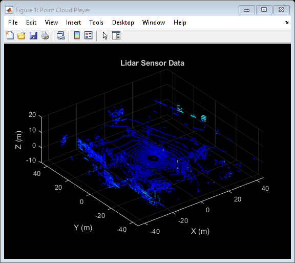
To understand what the scene contains, visualize the recorded data using streaming players. To visualize the GPS readings, usegeoplayer(Automated Driving Toolbox). To visualize lidar readings usingpcplayer.
% Create a geoplayer to visualize streaming geographic coordinateslatCenter = gpsSequence.Latitude(1); lonCenter = gpsSequence.Longitude(1); zoomLevel = 17; gpsPlayer = geoplayer(latCenter, lonCenter, zoomLevel);% Plot the full routeplotRoute(gpsPlayer, gpsSequence.Latitude, gpsSequence.Longitude);% Determine limits for the playerxlimits = [-45 45];% metersylimits = [-45 45]; zlimits = [-10 20];% Create a pcplayer to visualize streaming point clouds from lidar sensorlidarPlayer = pcplayer(xlimits, ylimits, zlimits);% Customize player axes labelsxlabel(lidarPlayer.Axes,'X (m)') ylabel(lidarPlayer.Axes,'Y (m)') zlabel(lidarPlayer.Axes,'Z (m)') title(lidarPlayer.Axes,'Lidar Sensor Data')% Align players on screenhelperAlignPlayers({gpsPlayer, lidarPlayer});% Outer loop over GPS readings (slower signal)forg = 1 : height(gpsSequence)-1% Extract geographic coordinates from timetablelatitude = gpsSequence.Latitude(g); longitude = gpsSequence.Longitude(g);% Update current position in GPS displayplotPosition(gpsPlayer, latitude, longitude);% Compute the time span between the current and next GPS readingtimeSpan = timerange(gpsSequence.Time(g), gpsSequence.Time(g+1));% Extract the lidar frames recorded during this time spanlidarFrames = lidarPointClouds(timeSpan, :);% Inner loop over lidar readings (faster signal)forl = 1 : height(lidarFrames)% Extract point cloudptCloud = lidarFrames.PointCloud(l);% Update lidar displayview(lidarPlayer, ptCloud);% Pause to slow down the displaypause(0.01)endend

Use Recorded Lidar Data to Build a Map
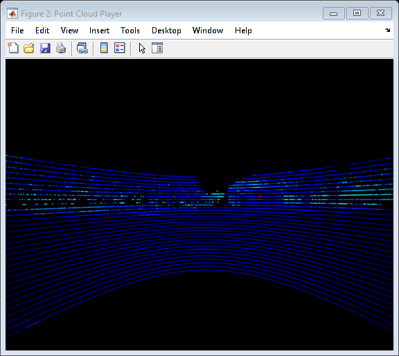
Lidars are powerful sensors that can be used for perception in challenging environments where other sensors are not useful. They provide a detailed, full 360 degree view of the environment of the vehicle.
% Hide playershide(gpsPlayer) hide(lidarPlayer)% Select a frame of lidar data to demonstrate registration workflowframeNum = 600; ptCloud = lidarPointClouds.PointCloud(frameNum);% Display and rotate ego view to show lidar datahelperVisualizeEgoView(ptCloud);
Lidars can be used to build centimeter-accurate HD maps, including HD maps of entire cities. These maps can later be used for in-vehicle localization. A typical approach to build such a map is to align successive lidar scans obtained from the moving vehicle and combine them into a single large point cloud. The rest of this example explores this approach to building a map.
Align lidar scans:Align successive lidar scans using a point cloud registration technique like the iterative closest point (ICP) algorithm or the normal-distributions transform (NDT) algorithm. See
pcregistericpandpcregisterndtfor more details about each algorithm. This example uses NDT, because it is typically more accurate, especially when considering rotations. Thepcregisterndtfunction returns the rigid transformation that aligns the moving point cloud with respect to the reference point cloud. By successively composing these transformations, each point cloud is transformed back to the reference frame of the first point cloud.Combine aligned scans:Once a new point cloud scan is registered and transformed back to the reference frame of the first point cloud, the point cloud can be merged with the first point cloud using
pcmerge.
Start by taking two point clouds corresponding to nearby lidar scans. To speed up processing, and accumulate enough motion between scans, use every tenth scan.
skipFrames = 10; frameNum = 100; fixed = lidarPointClouds.PointCloud(frameNum); moving = lidarPointClouds.PointCloud(frameNum + skipFrames);
Prior to registration, process the point cloud so as to retain structures in the point cloud that are distinctive. These pre-processing steps include the following:
Detect and remove the ground plane
Detect and remove ego-vehicle
These steps are described in more detail in theGround Plane and Obstacle Detection Using Lidar(Automated Driving Toolbox)example. In this example, thehelperProcessPointCloudhelper function accomplishes these steps.
fixedProcessed = helperProcessPointCloud(fixed); movingProcessed = helperProcessPointCloud(moving);
Display the raw and processed point clouds in top-view. Magenta points were removed during processing. These points correspond to the ground plane and ego vehicle.
hFigFixed = figure; pcshowpair(fixed, fixedProcessed) view(2);% Adjust view to show top-viewhelperMakeFigurePublishFriendly(hFigFixed);% Downsample the point clouds prior to registration. Downsampling improves% both registration accuracy and algorithm speed.downsamplePercent = 0.1; fixedDownsampled = pcdownsample(fixedProcessed,'random', downsamplePercent); movingDownsampled = pcdownsample(movingProcessed,'random', downsamplePercent);

After preprocessing the point clouds, register them using NDT. Visualize the alignment before and after registration.
regGridStep = 5; tform = pcregisterndt(movingDownsampled, fixedDownsampled, regGridStep); movingReg = pctransform(movingProcessed, tform);% Visualize alignment in top-view before and after registrationhFigAlign = figure; subplot(121) pcshowpair(movingProcessed, fixedProcessed) title('Before Registration') view(2) subplot(122) pcshowpair(movingReg, fixedProcessed) title('After Registration') view(2) helperMakeFigurePublishFriendly(hFigAlign);

Notice that the point clouds are well-aligned after registration. Even though the point clouds are closely aligned, the alignment is still not perfect.
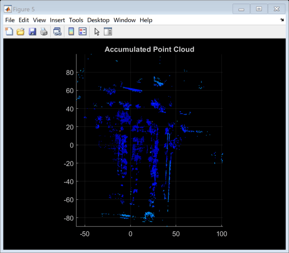
Next, merge the point clouds usingpcmerge.
mergeGridStep = 0.5; ptCloudAccum = pcmerge(fixedProcessed, movingReg, mergeGridStep); hFigAccum = figure; pcshow(ptCloudAccum) title('Accumulated Point Cloud') view(2) helperMakeFigurePublishFriendly(hFigAccum);
Now that the processing pipeline for a single pair of point clouds is well-understood, put this together in a loop over the entire sequence of recorded data. ThehelperLidarMapBuilderclass puts all this together. TheupdateMapmethod of the class takes in a new point cloud and goes through the steps detailed previously:
Processing the point cloud by removing the ground plane and ego vehicle, using the
processPointCloudmethod.Downsampling the point cloud.
Estimating the rigid transformation required to merge the previous point cloud with the current point cloud.
Transforming the point cloud back to the first frame.
合并的点云积累点cloud map.
Additionally, theupdateMapmethod also accepts an initial transformation estimate, which is used to initialize the registration. A good initialization can significantly improve results of registration. Conversely, a poor initialization can adversely affect registration. Providing a good initialization can also improve the execution time of the algorithm.
A common approach to providing an initial estimate for registration is to use a constant velocity assumption. Use the transformation from the previous iteration as the initial estimate.
TheupdateDisplaymethod additionally creates and updates a 2-D top-view streaming point cloud display.
% Create a map builder objectmapBuilder = helperLidarMapBuilder('DownsamplePercent', downsamplePercent);% Set random number seedrng(0); closeDisplay = false; numFrames = height(lidarPointClouds); tform = rigidtform3d;forn = 1 : skipFrames : numFrames - skipFrames% Get the nth point cloudptCloud = lidarPointClouds.PointCloud(n);% Use transformation from previous iteration as initial estimate for% current iteration of point cloud registration. (constant velocity)initTform = tform;% Update map using the point cloudtform = updateMap(mapBuilder, ptCloud, initTform);% Update map displayupdateDisplay(mapBuilder, closeDisplay);end

Point cloud registration alone builds a map of the environment traversed by the vehicle. While the map may appear locally consistent, it might have developed significant drift over the entire sequence.
Use the recorded GPS readings as a ground truth trajectory, to visually evaluate the quality of the built map. First convert the GPS readings (latitude, longitude, altitude) to a local coordinate system. Select a local coordinate system that coincides with the origin of the first point cloud in the sequence. This conversion is computed using two transformations:
Convert the GPS coordinates to local Cartesian East-North-Up coordinates using the
latlon2local(Automated Driving Toolbox)function. The GPS location from the start of the trajectory is used as the reference point and defines the origin of the local x,y,z coordinate system.Rotate the Cartesian coordinates so that the local coordinate system is aligned with the first lidar sensor coordinates. Since the exact mounting configuration of the lidar and GPS on the vehicle are not known, they are estimated.
% Select reference point as first GPS readingorigin = [gpsSequence.Latitude(1), gpsSequence.Longitude(1), gpsSequence.Altitude(1)];% Convert GPS readings to a local East-North-Up coordinate system[xEast, yNorth, zUp] = latlon2local(gpsSequence.Latitude, gpsSequence.Longitude,...gpsSequence.Altitude, origin);% Estimate rough orientation at start of trajectory to align local ENU% system with lidar coordinate systemtheta = median(atan2d(yNorth(1:15), xEast(1:15))); R = [ cosd(90-theta) sind(90-theta) 0; -sind(90-theta) cosd(90-theta) 0; 0 0 1];% Rotate ENU coordinates to align with lidar coordinate systemgroundTruthTrajectory = [xEast, yNorth, zUp] * R;
Superimpose the ground truth trajectory on the built map.
hold(mapBuilder.Axes,'on') scatter(mapBuilder.Axes, groundTruthTrajectory(:,1), groundTruthTrajectory(:,2),...'green','filled'); helperAddLegend(mapBuilder.Axes,...{“地图点”,'Estimated Trajectory','Ground Truth Trajectory'});
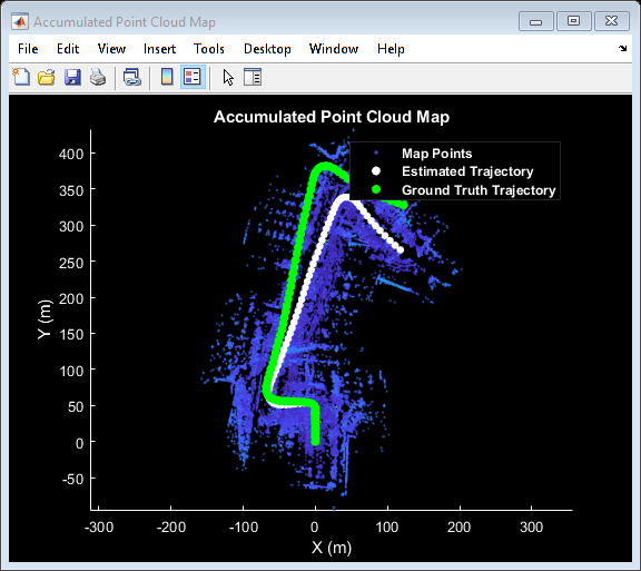
After the initial turn, the estimated trajectory veers off the ground truth trajectory significantly. The trajectory estimated using point cloud registration alone can drift for a number of reasons:
Noisy scans from the sensor without sufficient overlap
Absence of strong enough features, for example, near long roads
Inaccurate initial transformation, especially when rotation is significant.
% Close map displayupdateDisplay(mapBuilder, true);
Use IMU Orientation to Improve Built Map
An IMU is an electronic device mounted on a platform. IMUs contain multiple sensors that report various information about the motion of the vehicle. Typical IMUs incorporate accelerometers, gyroscopes, and magnetometers. An IMU can provide a reliable measure of orientation.
Use the IMU readings to provide a better initial estimate for registration. The IMU-reported sensor readings used in this example have already been filtered on the device.
% Reset the map builder to clear previously built mapreset(mapBuilder);% Set random number seedrng(0); initTform = rigidtform3d;forn = 1 : skipFrames : numFrames - skipFrames% Get the nth point cloudptCloud = lidarPointClouds.PointCloud(n);ifn > 1% Since IMU sensor reports readings at a much faster rate, gather% IMU readings reported since the last lidar scan.prevTime = lidarPointClouds.Time(n - skipFrames); currTime = lidarPointClouds.Time(n); timeSinceScan = timerange(prevTime, currTime); imuReadings = imuOrientations(timeSinceScan,'Orientation');% Form an initial estimate using IMU readingsinitTform = helperComputeInitialEstimateFromIMU(imuReadings, tform);end% Update map using the point cloudtform = updateMap(mapBuilder, ptCloud, initTform);% Update map displayupdateDisplay(mapBuilder, closeDisplay);end% Superimpose ground truth trajectory on new maphold(mapBuilder.Axes,'on') scatter(mapBuilder.Axes, groundTruthTrajectory(:,1), groundTruthTrajectory(:,2),...'green','filled'); helperAddLegend(mapBuilder.Axes,...{“地图点”,'Estimated Trajectory','Ground Truth Trajectory'});% Capture snapshot for publishingsnapnow;% Close open figuresclose([hFigFixed, hFigAlign, hFigAccum]); updateDisplay(mapBuilder, true);
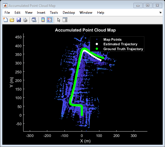
Using the orientation estimate from IMU significantly improved registration, leading to a much closer trajectory with smaller drift.
Supporting Functions
helperAlignPlayersaligns a cell array of streaming players so they are arranged from left to right on the screen.
functionhelperAlignPlayers(players) validateattributes(players, {'cell'}, {'vector'}); hasAxes = cellfun(@(p)isprop(p,'Axes'),players,'UniformOutput', true);if~all(hasAxes) error('Expected all viewers to have an Axes property');endscreenSize = get(groot,'ScreenSize'); screenMargin = [50, 100]; playerSizes = cellfun(@getPlayerSize, players,'UniformOutput', false); playerSizes = cell2mat(playerSizes); maxHeightInSet = max(playerSizes(1:3:end));% Arrange players vertically so that the tallest player is 100 pixels from% the top.location = round([screenMargin(1), screenSize(4)-screenMargin(2)-maxHeightInSet]);forn = 1 : numel(players) player = players{n}; hFig = ancestor(player.Axes,'figure'); hFig.OuterPosition(1:2) = location;% Set up next location by going rightlocation = location + [50+hFig.OuterPosition(3), 0];endfunctionsz = getPlayerSize(viewer)% Get the parent figure containerh = ancestor(viewer.Axes,'figure'); sz = h.OuterPosition(3:4);endend
helperVisualizeEgoViewvisualizes point cloud data in the ego perspective by rotating about the center.
functionplayer = helperVisualizeEgoView(ptCloud)% Create a pcplayer objectxlimits = ptCloud.XLimits; ylimits = ptCloud.YLimits; zlimits = ptCloud.ZLimits; player = pcplayer(xlimits, ylimits, zlimits);% Turn off axes linesaxis(player.Axes,'off');% Set up camera to show ego viewcamproj(player.Axes,'perspective'); camva(player.Axes, 90); campos(player.Axes, [0 0 0]); camtarget(player.Axes, [-1 0 0]);% Set up a transformation to rotate by 5 degreesθ= 5;eulerAngles =[0 0θ];翻译= [0 0 0]; rotateByTheta = rigidtform3d(eulerAngles, translation);forn = 0 : theta : 359% Rotate point cloud by thetaptCloud = pctransform(ptCloud, rotateByTheta);% Display point cloudview(player, ptCloud); pause(0.05)endend
helperProcessPointCloudprocesses a point cloud by removing points belonging to the ground plane or ego vehicle.
functionptCloudProcessed = helperProcessPointCloud(ptCloud)% Check if the point cloud is organizedisOrganized = ~ismatrix(ptCloud.Location);% If the point cloud is organized, use range-based flood fill algorithm% (segmentGroundFromLidarData). Otherwise, use plane fitting.groundSegmentationMethods = ["planefit","rangefloodfill"]; method = groundSegmentationMethods(isOrganized+1);ifmethod =="planefit"% Segment ground as the dominant plane, with reference normal vector% pointing in positive z-direction, using pcfitplane. For organized% point clouds, consider using segmentGroundFromLidarData instead.maxDistance = 0.4;% metersmaxAngDistance = 5;% degreesrefVector = [0, 0, 1];% z-direction[~,groundIndices] = pcfitplane(ptCloud, maxDistance, refVector, maxAngDistance);elseifmethod =="rangefloodfill"% Segment ground using range-based flood fill.groundIndices = segmentGroundFromLidarData(ptCloud);elseerror("Expected method to be 'planefit' or 'rangefloodfill'")end% Segment ego vehicle as points within a given radius of sensorsensorLocation = [0, 0, 0]; radius = 3.5; egoIndices = findNeighborsInRadius(ptCloud, sensorLocation, radius);% Remove points belonging to ground or ego vehicleptsToKeep = true(ptCloud.Count, 1); ptsToKeep(groundIndices) = false; ptsToKeep(egoIndices) = false;% If the point cloud is organized, retain organized structureifisOrganized ptCloudProcessed = select(ptCloud, find(ptsToKeep),'OutputSize','full');elseptCloudProcessed = select(ptCloud, find(ptsToKeep));endend
helperComputeInitialEstimateFromIMUestimates an initial transformation for NDT using IMU orientation readings and previously estimated transformation.
functiontform = helperComputeInitialEstimateFromIMU(imuReadings, prevTform)% Initialize transformation using previously estimated transformtform = prevTform;% If no IMU readings are available, returnifheight(imuReadings) <= 1return;end% IMU orientation readings are reported as quaternions representing the% rotational offset to the body frame. Compute the orientation change% between the first and last reported IMU orientations during the interval% of the lidar scan.q1 = imuReadings.Orientation(1); q2 = imuReadings.Orientation(end);% Compute rotational offset between first and last IMU reading by% - Rotating from q2 frame to body frame% - Rotating from body frame to q1 frameq = q1 * conj(q2);% Convert to Euler anglesyawPitchRoll = euler(q,'ZYX','point');% Discard pitch and roll angle estimates. Use only heading angle estimate% from IMU orientation.yawPitchRoll(2:3) = 0;% Convert back to rotation matrixq = quaternion(yawPitchRoll,'euler','ZYX','point'); R = rotmat(q,'point');% Use computed rotationtform.T(1:3, 1:3) = R';end
helperAddLegendadds a legend to the axes.
functionhelperAddLegend(hAx, labels)% Add a legend to the axeshLegend = legend(hAx, labels{:});% Set text color and font weighthLegend.TextColor = [1 1 1]; hLegend.FontWeight ='bold';end
helperMakeFigurePublishFriendlyadjusts figures so that screenshot captured by publish is correct.
functionhelperMakeFigurePublishFriendly(hFig)if~isempty(hFig) && isvalid(hFig) hFig.HandleVisibility ='callback';endend
See Also
Functions
Objects
pcplayer|geoplayer(Automated Driving Toolbox)|pointCloud
Related Topics
- Build a Map from Lidar Data Using SLAM
- Ground Plane and Obstacle Detection Using Lidar(Automated Driving Toolbox)
External Websites
You can also select a web site from the following list:
Americas
- América Latina(Español)
- Canada(English)
- United States(English)
Europe
- Belgium(English)
- Denmark(English)
- Deutschland(Deutsch)
- España(Español)
- Finland(English)
- France(Français)
- Ireland(English)
- Italia(Italiano)
- Luxembourg(English)
- Netherlands(English)
- Norway(English)
- Österreich(Deutsch)
- Portugal(English)
- Sweden(English)
- Switzerland
- United Kingdom(English)