What Is Multiresolution Analysis?

Signals often consist of multiple physically meaningful components. Quite often, you want to study one or more of these components in isolation on the same time scale as the original data.Multiresolution analysisrefers to breaking up a signal into components, which produce the original signal exactly when added back together. To be useful for data analysis, how the signal is decomposed is important. The components ideally decompose the variability of the data into physically meaningful and interpretable parts. The termmultiresolution analysisis often associated with wavelets or wavelet packets, but there are non-wavelet techniques which also produce useful MRAs.

As a motivating example of the insights you can gain from an MRA, consider the following synthetic signal. The signal is sampled at 1000 Hz for one second.

Fs = 1e3; t = 0:1/Fs:1-1/Fs; comp1 = cos(2*pi*200*t).*(t>0.7); comp2 = cos(2*pi*60*t).*(t>=0.1 & t<0.3); trend = sin(2*pi*1/2*t); rngdefaultwgnNoise = 0.4*randn(size(t)); x = comp1+comp2+trend+wgnNoise; plot(t,x) xlabel('Seconds') ylabel('Amplitude') title('Synthetic Signal')

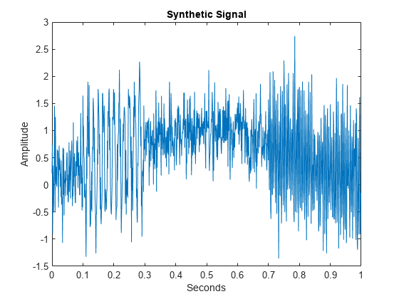
The signal is explicitly composed of three main components: a time-localized oscillation with a frequency of 60 cycles/second, a time-localized oscillation with a frequency of 200 cycles/second, and a trend term. The trend term here is also sinusoidal but has a frequency of 1/2 cycle per second, so it completes only 1/2 cycle in the one-second interval. The 60 cycles/second or 60 Hz oscillation occurs between 0.1 and 0.3 seconds, while the 200 Hz oscillation occurs between 0.7 and 1 second.

Not all of this is immediately evident from the plot of the raw data because these components are mixed.

Now, plot the signal from a frequency point of view.

xdft = fft(x); N = numel(x); xdft = xdft(1:numel(xdft)/2+1); freq = 0:Fs/N:Fs/2; plot(freq,20*log10(abs(xdft))) xlabel('Cycles/second') ylabel('dB') gridon

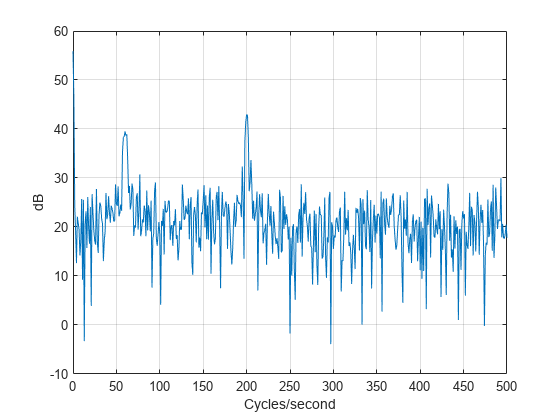
From the frequency analysis, it is much easier for us to discern the frequencies of the oscillatory components, but we have lost their time-localized nature. It is also difficult to visualize the trend in this view.

To gain some simultaneous time and frequency information, we can use a time-frequency analysis technique like the continuous wavelet transform (cwt).

cwt(x,Fs)

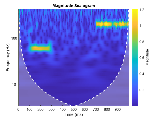
Now you see the time extents of the 60 Hz and 200 Hz components. However, we still do not have any useful visualization of the trend.

The time-frequency view provides useful information, but in many situations you would like to separate out components of the signal in time and examine them individually. Ideally, you want this information to be available on the same time scale as the original data.

Multiresolution analysis accomplishes this. In fact, a useful way to think about multiresolution analysis is that it provides a way of avoiding the need for time-frequency analysis while allowing you to work directly in the time domain.

Separating Signal Components in Time

Real-world signals are a mixture of different components. Often you are only interested in a subset of these components. Multiresolution analysis allows you to narrow your analysis by separating the signal into components at differentresolutions。

Extracting signal components at different resolutions amounts to decomposing variations in the data on different time scales, or equivalently in different frequency bands (different rates of oscillation). Accordingly, you can visualize signal variability at different scales, or frequency bands simultaneously.

Analyze and plot the synthetic signal using a wavelet MRA. The signal is analyzed at eight resolutions or levels.

mra = modwtmra(modwt(x,8)); helperMRAPlot(x,mra,t,'wavelet','Wavelet MRA',[2 3 4 9])

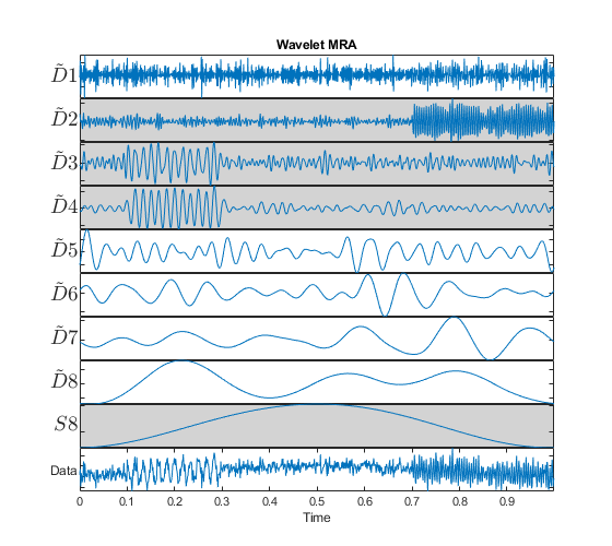
Without explaining what the notations on the plot mean, let us use our knowledge of the signal and try to understand what this wavelet MRA is showing us. If you start from the uppermost plot and proceed down until you reach the plot of the original data, you see that the components become progressively smoother. If you prefer to think about data in terms of frequency, the frequencies contained in the components are becoming lower. Recall that the original signal had three main components, a high frequency oscillation at 200 Hz, a lower frequency oscillation of 60 Hz, and a trend term, all corrupted by additive noise.

If you look at the $$\underset{}{\overset{\sim }{D}}2$$plot, you can see that the time-localized high frequency component is isolated there. You can see and investigate this important signal feature essentially in isolation. The next two plots contain the lower frequency oscillation. This is an important aspect of multiresolution analysis, namely important signal components may not end up isolated in one MRA component, but they are rarely located in more than two. Finally, we see the $$S8$$plot contains the trend term. For convenience, the color of the axes in those components has been changed to highlight them in the MRA. If you prefer to visualize this plot or subsequent ones without the highlighting, leave out the last numeric input tohelperMRAPlot。

The wavelet MRA uses fixed functions calledwaveletsto separate the signal components. Thekth wavelet MRA component, denoted by $$\underset{}{\overset{\sim }{D}}k$$在前面的情节,可以被视为一个filtering of the signal into frequency bands of the form $[\frac{1}{2^{k+1}\Delta t},\frac{1}{2^k\Delta t}]$where $\Delta t$is the sampling period, or sampling interval. The final smooth component, denoted in the plot by $$SL$$, where $$L$$is the level of the MRA, captures the frequency band $[0,\frac{1}{2^{L+1}\Delta t}]$。这个近似的准确性取决于the wavelet used in the MRA. See [5] for detailed descriptions of wavelet and wavelet packet MRAs.

However, there are other MRA techniques to consider.

Theempirical mode decomposition(EMD) is a data-adaptive multiresolution technique. EMD recursively extracts different resolutions from the data without the use of fixed functions or filters. EMD regards a signal as consisting of afastoscillation superimposed on aslowerone. After the fast oscillation is extracted, the process treats the remaining slower component as the new signal and again regards it as a fast oscillation superimposed on a slower one. The process continues until some stopping criterion is reached. While EMD does not use fixed functions like wavelets to extract information, the EMD approach is conceptually very similar to the wavelet method of separating the signal intodetailsandapproximationsand then separating the approximation again into details and an approximation. The MRA components in EMD are referred to asintrinsic mode functions(IMF). See [4] for a detailed treatment of EMD.

Plot the EMD analysis of the same signal.

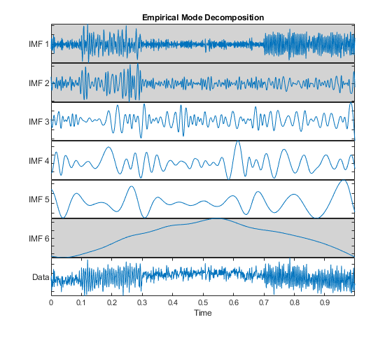
[imf_emd,resid_emd] = emd(x); helperMRAPlot(x,imf_emd,t,'emd','Empirical Mode Decomposition',[1 2 3 6])

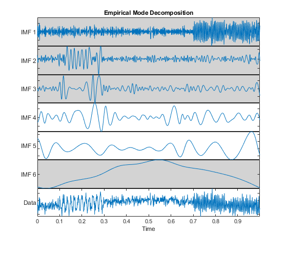
While the number of MRA components is different, the EMD and wavelet MRAs produce a similar picture of the signal. This is not accidental. See [2] for a description of the similarities between the wavelet transform and EMD.

In the EMD decomposition, the high-frequency oscillation is localized to the first intrinsic mode function (IMF 1). The lower frequency oscillation is localized largely to IMF 2, but you can see some effect also in IMF 3. The trend component in IMF 6 is very similar to the trend component extracted by the wavelet technique.

Yet another technique for adaptive multiresolution analysis isvariational mode decomposition(VMD). Like EMD, VMD attempts to extract intrinsic mode functions, or modes of oscillation from the signal without using fixed functions for analysis. But EMD and VMD determine the modes in very different ways. EMD works recursively on the time-domain signal to extract progressively lower frequency IMFs. VMD starts by identifying signal peaks in the frequency domain and extracts all modes concurrently. See [1] for a treatment of VMD.

[imf_vmd,resid_vmd] = vmd(x); helperMRAPlot(x,imf_vmd,t,'vmd','Variational Mode Decomposition',[2 4 5])

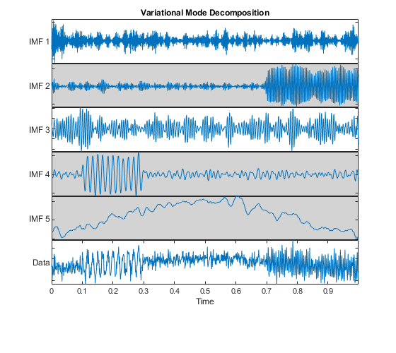
The key thing to note is that similar to the wavelet and EMD decompositions, VMD segregates the three components of interest into completely separate modes or into a small number of adjacent modes. All three techniques allow you to visualize signal components on the same time scale as the original signal.

There is a data-adaptive technique which actually constructs wavelet filters based on the frequency content of the data. This technique is theempirical wavelet transform(EWT) [3］．EMD的一个主要的批评是,它definition is purely algorithmic. As a result, it is not readily amenable to mathematical analysis. EWT on the other hand actually constructs Meyer wavelets based on the frequency content of the analyzed signal. Accordingly, the results of EWT are amenable to mathematical analysis because the filters used in the analysis are available to the user. Repeat the analysis of the the synthetic signal using the EWT.

[mra_ewt,cfs,wfb,info] = ewt(x,'MaxNumPeaks',5); helperMRAPlot(x,mra_ewt,t,'EWT','Empirical Wavelet Transform',[1 2 3 5])

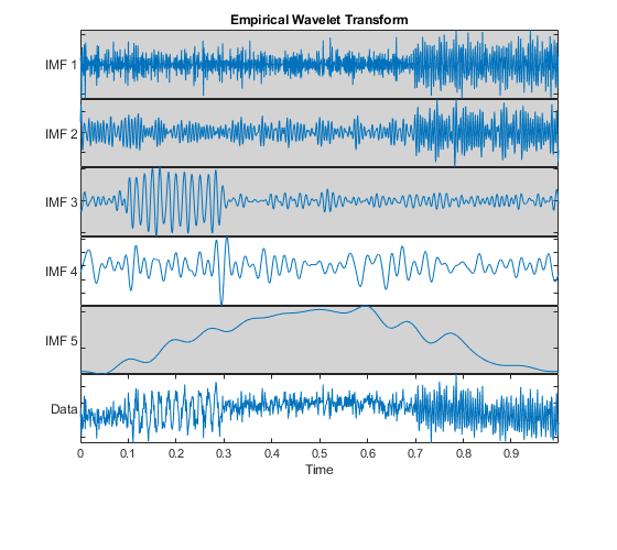
Similar to the previous EMD and wavelet MRA techniques, the EWT has isolated the oscillatory components and trend to a few intrinsic mode functions. In contrast to EMD however, the filters used to perform the analysis and their passband information are available to the user.

Nf = length(x)/2+1; cf = mean(info.FilterBank.Passbands,2); f = 0:Fs/length(x):Fs-Fs/length(x); clf ax = newplot; plot(ax,f(1:Nf),wfb(1:Nf,:)) ax.XTick = sort(cf.*Fs); ax.XTickLabel = ax.XTick; xlabel('Hz') gridontitle('Empirical Meyer Wavelets')

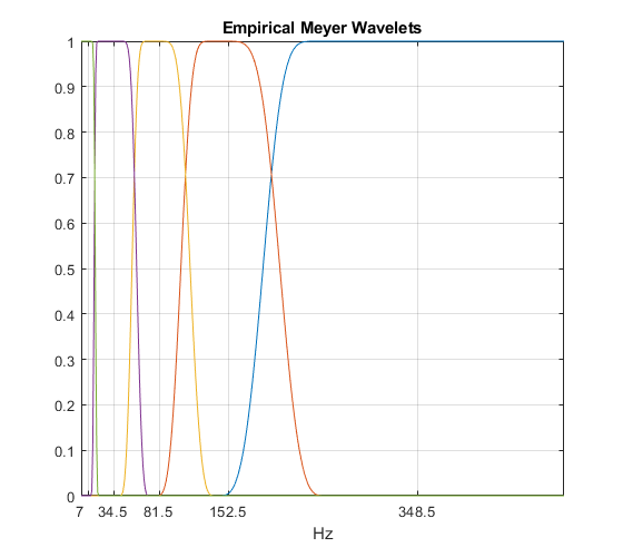
Another advantage of the EWT technique is that the analysis coefficients preserve the energy of the original signal. This property is shared by the non-adaptive wavelet techniques, but is not found in the non-wavelet adaptive techniques.

EWTEnergy = sum(vecnorm(cfs,2).^2)

EWTEnergy = 875.5768

sigEnergy = norm(x,2)^2

sigEnergy = 875.5768

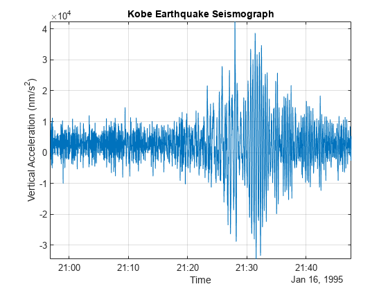
For a real-world example of useful component separation, consider a seismograph (vertical acceleration, $$\text{nm}/{\text{s}}^2$$) of the Kobe earthquake, recorded at Tasmania University, Hobart, Australia on 16 January 1995 beginning at 20:56:51 (GMT) and continuing for 51 minutes at 1 second intervals.

loadKobeTimeTableT = KobeTimeTable.t; kobe = KobeTimeTable.kobe; figure plot(T,kobe) title('Kobe Earthquake Seismograph') ylabel('Vertical Acceleration (nm/s^2)') xlabel('Time') axistightgridon

Obtain and plot a wavelet MRA of the data.

mraKobe = modwtmra(modwt(kobe,8)); figure helperMRAPlot(kobe,mraKobe,T,'Wavelet','Wavelet MRA Kobe Earthquake',[4 5])

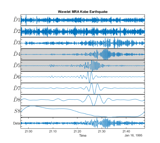
The plot shows the separation of primary and delayed secondary wave components in MRA components $\underset{}{\overset{\sim }{D}}4$and $\underset{}{\overset{\sim }{D}}5$。Components in a seismic wave travel at different velocities with primary (compressional) waves traveling faster than secondary (shear) waves. MRA techniques can enable you to study these components in isolation on the original time scale.

Reconstructing Signals from MRA

The point of separating signals into components is often to remove certain components or mitigate their effect on the signal. Crucial to MRA techniques is the ability to reconstruct the original signal.

First, let us demonstrate that all these multiresolution techniques allow you to perfectly reconstruct the signal from the components.

sigrec_wavelet = sum(mra); sigrec_emd = sum(imf_emd,2)+resid_emd; sigrec_vmd = sum(imf_vmd,2)+resid_vmd; figure subplot(3,1,1) plot(t,sigrec_wavelet); title('Wavelet reconstruction'); set(gca,'XTickLabel',[]); ylabel('Amplitude'); subplot(3,1,2); plot(t,sigrec_emd); title('EMD reconstruction'); set(gca,'XTickLabel',[]); ylabel('Amplitude'); subplot(3,1,3) plot(t,sigrec_vmd); title('VMD reconstruction'); ylabel('Amplitude'); xlabel('Time');

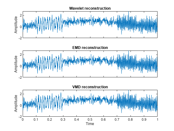
The maximum reconstruction error on a sample-by-sample basis for each of the methods is on the order of $10^{-12}$or smaller, indicating they are perfect reconstruction methods. Because the sum of the MRA components reconstructs the original signal, it stands to reason that including or excluding a subset of components could produce a useful approximation.

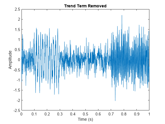
Return to our original wavelet MRA of the synthetic signal and suppose that you were not interested in in the trend term. Because the trend term is localized in the last MRA component, just exclude that component from the reconstruction.

sigWOtrend = sum(mra(1:end-1,:)); figure plot(t,sigWOtrend) xlabel('Time (s)') ylabel('Amplitude') title('Trend Term Removed')

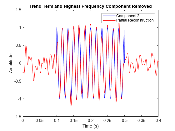
To remove other components, you can create a logical vector withfalsevalues in components you do not wish to include. Here we remove the trend and highest frequency component along with the first MRA component (which looks to be largely noise). Plot the actual second signal component (60 Hz) along with the reconstruction for comparison.

include = true(size(mra,1),1); include([1 2 9]) = false; ts = sum(mra(include,:)); plot(t,comp2,'b') holdonplot(t,ts,'r') title('Trend Term and Highest Frequency Component Removed') xlabel('Time (s)') ylabel('Amplitude') legend('Component 2','Partial Reconstruction') xlim([0.0 0.4])

In the previous example, we treated the trend term as a nuisance component to be removed. There are a number of applications where the trend may be the primary component of interest. Let us visualize the trend terms extracted by our three example MRAs.

figure plot(t,trend,'LineWidth',2) holdonplot(t,[mra(end,:)' imf_vmd(:,end) imf_emd(:,end) mra_ewt(:,end)]) gridonlegend('Trend','Wavelet','VMD','EMD','EWT') ylabel('Amplitude') xlabel('Time (s)') title('Trend in three MRAs')

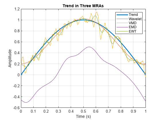
注意,这一趋势是最accuratel更平稳y captured by the wavelet technique. EMD finds a smooth trend term, but it is shifted with respect to the true trend amplitude while the VMD technique seems inherently more biased toward finding oscillations than the wavelet and EMD techniques. The implications of this are further discussed in theMRA Techniques — Advantages and Disadvantagessection.

Detecting Transient Changes Using MRA

In the previous examples, the role of multiresolution analysis in the detection of oscillatory components in the data and an overall trend was emphasized. However, these are not the only signal features that can be analyzed using multiresolution analysis. MRA can also help localize and detect transient features in a signal like impulsive events, or reductions or increases in variability in certain components. Changes in variability localized to certain scales or frequency bands often indicate significant changes in the process generating the data. These changes are frequently more easily visualized in the MRA components than in the raw data.

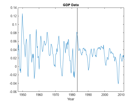
To illustrate this, consider the quarterly chain-weighted U.S. real gross domestic product (GDP) data for 1947Q1 to 2011Q4. Quarterly samples correspond to a sampling frequency of 4 samples/year. The vertical black line marks the beginning of the "Great Moderation" signifying a period of decreased macroeconomic volatility in the U.S. beginning in the mid-1980s. Note that this is difficult to discern looking at the raw data.

loadGDPDatafigure plot(year,realgdp) holdonplot([year(146) year(146)],[-0.06 0.14],'k') title('GDP Data') xlabel('Year') holdoff

Obtain a wavelet MRA of the GDP data. Plot the finest resolution MRA component with the period of the great moderation marked. Because the wavelet MRA is obtained using fixed filters, we can associate the finest-scale MRA component with frequencies of 1 cycle per year to 2 cycles per year. A component which oscillated with a period of two quarters has a frequency of 2 cycles per year. In this case, the finest-resolution MRA component captures changes in the GDP that occur between adjacent two-quarter intervals to changes that occur from quarter to quarter.

mra = modwtmra(modwt(realgdp,'db2')); figure plot(year,mra(1,:)) holdonplot([year(146) year(146)],[-0.015 0.015],'k') title('Wavelet MRA - Quarter-to-Quarter Changes') xlabel('Year') holdoff

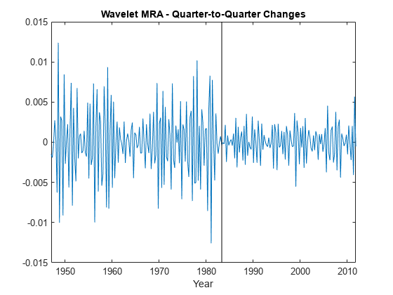
The reduction in variability, or in economic terms volatility, is much more readily apparent in the finest resolution MRA component than in the raw data. Techniques to detect changes in variance like the MATLABfindchangepts(Signal Processing Toolbox)often work better on MRA components than on the raw data.

MRA Techniques — Advantages and Disadvantages

In this example, we discussed wavelet and data-adaptive techniques for multiresolution analysis. What are some of the advantages and disadvantages of the various techniques? In other words, for what applications might I choose one over the other? Let us start with wavelets. The wavelet techniques in this example use fixed filters to obtain the MRA. This means that the wavelet MRA has a well-defined mathematical explanation and we can predict the behavior of the MRA. We are also able to tie events in the MRA to specific time scales in the data as was done in the GDP example. The disadvantage is that the wavelet transform divides the signal into octave bands (a reduction in center frequency by 1/2 in each component) so that at high center frequencies the bandwidths are much larger than those at lower frequencies. This means two closely spaced high frequency oscillations can easily end up in the same MRA component with a wavelet technique.

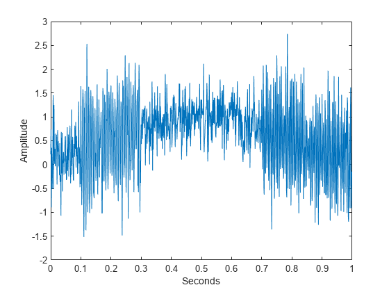
Repeat the first synthetic example but move the two oscillatory components within one octave of each other.

Fs = 1e3; t = 0:1/Fs:1-1/Fs; comp1 = cos(2*pi*150*t).*(t>=0.1 & t<0.3); comp2 = cos(2*pi*200*t).*(t>0.7); trend = sin(2*pi*1/2*t); rngdefault; wgnNoise = 0.4*randn(size(t)); x = comp1+comp2+trend+wgnNoise; plot(t,x) xlabel('Seconds') ylabel('Amplitude')

Repeat and plot the wavelet MRA.

mra = modwtmra(modwt(x,8)); helperMRAPlot(x,mra,t,'wavelet','Wavelet MRA',[2 9])

Now we see that $\underset{}{\overset{\sim }{D}}2$contains both the 150 Hz and 200 Hz components. If you repeat this analysis using EMD, you see the same result.

Now let us use the VMD.

[imf_vmd,~,info_vmd] = vmd(x); helperMRAPlot(x,imf_vmd,t,'vmd','VMD',[1 2 3 5]);

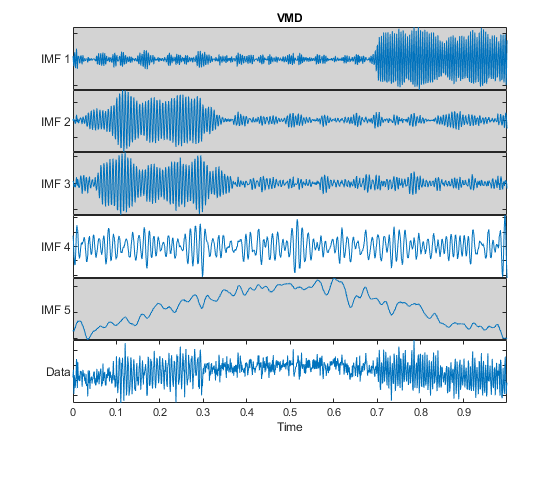
VMD is able to separate the two components. The high frequency oscillation localized to IMF 1, while the second component is spread over two adjacent IMFs. If you look at the estimated central frequencies of the VMD modes, the technique has localized the first two components around 200 and 150 Hz. The third IMF has a center frequency close to 150 Hz, which is why we see the second component in two MRA components.

info_vmd.CentralFrequencies*Fs

ans =5×1202.7204 153.3278 148.8022 84.2802 0.2667

VMD is able to do this because it starts by identifying candidate center frequencies for IMFs by looking at a frequency-domain analysis of the data.

While the wavelet MRA is not able to separate the two high-frequency components, there is an additionalwavelet packetMRA which can.

wpt = modwptdetails(x,3); helperMRAPlot(x,flip(wpt),t,'wavelet','Wavelet Packet MRA',[5 6 8]);

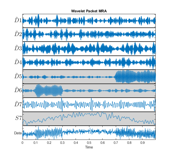
Now you see the two oscillations are separated in $\underset{}{\overset{\sim }{D}}5$and $\underset{}{\overset{\sim }{D}}6$。From this example we can extract a general rule. If an initial wavelet or EMD decomposition shows components with apparently different rates of oscillation in the same component, consider VMD or a wavelet packet MRA. If you suspect that your data has high frequency components close together in frequency, VMD or a wavelet packet approach will generally work better than a wavelet or EMD approach.

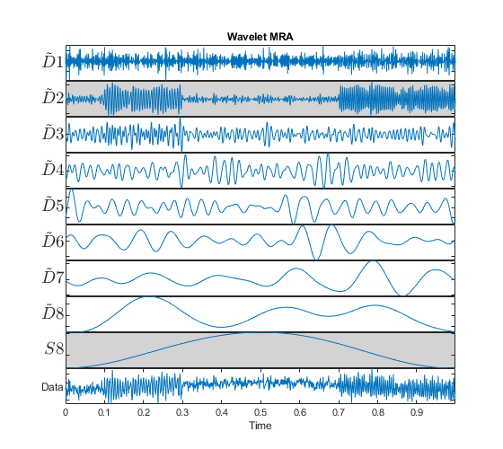
Recall the problem of extracting a smooth trend. Repeat both the wavelet MRA and the EMD.

mra = modwtmra(modwt(x,8)); helperMRAPlot(x,mra,t,'wavelet','Wavelet MRA',[2 9])

imf_emd = emd(x); helperMRAPlot(x,imf_emd,t,'EMD','Empirical Mode Decomposition',[1 2 6])

The trends extracted by the wavelet and EMD techniques are closer to the true trend than those extracted by VMD and the wavelet packet technique. VMD is inherently biased toward finding narrowband oscillatory components. This is a strength of VMD in detecting closely spaced oscillations, but a disadvantage when extracting smooth trends in the data. The same is true of wavelet packet MRAs when the decomposition goes beyond a few levels. This leads to a second general recommendation. If you are interested in characterizing a smooth trend in your data for identification or removal, try a wavelet or EMD technique.

What about detecting transient changes as we saw in the GDP data? Let us repeat the GDP analysis using VMD.

[imf_vmd,~,vmd_info] = vmd(realgdp); figure subplot(2,1,1) plot(year,realgdp) title('Real GDP'); holdonplot([year(146) year(146)],[-0.1 0.15],'k') holdoffsubplot(2,1,2) plot(year,imf_vmd(:,1)); title('First VMD IMF'); xlabel('Year') holdonplot([year(146) year(146)],[-0.02 0.02],'k') holdoff

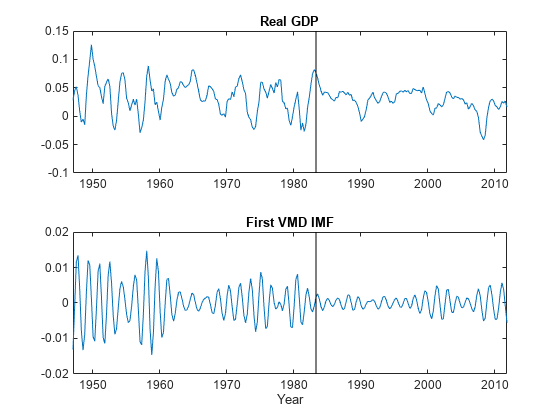
While the highest-frequency VMD component also appears to show some reduction in variability beginning in the mid-1980s, it is not as readily apparent as in the wavelet MRA. Because the VMD technique is biased toward finding oscillations, there is substantial ringing in the first VMD IMF which obscures the volatility changes.

Repeat this analysis using EMD.

imf_emd = emd(realgdp); figure subplot(2,1,1) plot(year,realgdp) title('Real GDP'); holdonplot([year(146) year(146)],[-0.1 0.15],'k') holdoffsubplot(2,1,2) plot(year,imf_emd(:,1)); title('First EMD IMF') xlabel('Year') holdonplot([year(146) year(146)],[-0.06 0.05],'k') holdoff

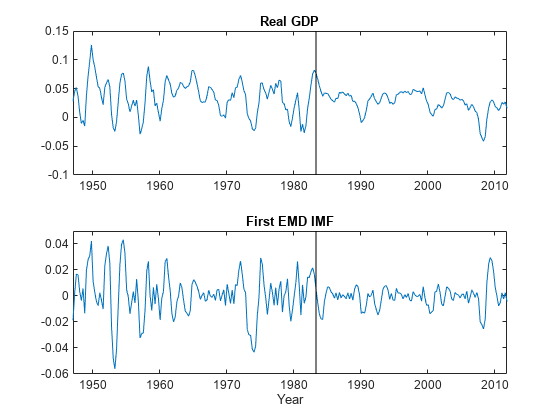
The EMD technique is less useful in finding the change in volatility (variance). In this case, the fixed functions using in the wavelet MRA were more advantageous than the data adaptive techniques.

This leads to our final general rule. If you are interested in detecting transient changes in a signal like impulsive events are reductions and increases in variability, try a wavelet technique.

Conclusions

This example showed how multiresolution decomposition techniques such as wavelet, wavelet packet, empirical mode decomposition, empirical wavelet, and variational mode decomposition allow you to study signal components in relative isolation on the same time scale as the original data. Each technique has proven itself powerful in a number of applications. The example has given a few rules of thumb to get you started, but these should not be regarded as absolute. The following table recaps properties of the MRA techniques presented here along with some general rules of thumb. Two plusses denote a particular strength, one plus indicates that the technique is applicable, but not a particular strength. For a binary property like the preservation of energy in the analysis, a check mark indicates the technique has this property and an "x" indicates the property is absent.

WithSignal Multiresolution Analyzer, you can perform multiresolution analysis on a signal, obtain metrics on various MRA components, experiment with partial reconstructions, and generate MATLAB scripts to reproduce the analysis at the command line.

References

[1] Dragomiretskiy, Konstantin, and Dominique Zosso. “Variational Mode Decomposition.”IEEE Transactions on Signal Processing62, no. 3 (February 2014): 531–44.https://doi.org/10.1109/TSP.2013.2288675。

[2] Flandrin, P., G. Rilling, and P. Goncalves. “Empirical Mode Decomposition as a Filter Bank.”IEEE Signal Processing Letters11, no. 2 (February 2004): 112–14.https://doi.org/10.1109/LSP.2003.821662。

[3] Giles, J. "Empirical wavelet transform",IEEE Transactions on Signal Processing,vol. 61, no. 16 (May 2013): 3999 - 4010.

[4] Huang, Norden E., Zheng Shen, Steven R. Long, Manli C. Wu, Hsing H. Shih, Quanan Zheng, Nai-Chyuan Yen, Chi Chao Tung, and Henry H. Liu. “The Empirical Mode Decomposition and the Hilbert Spectrum for Nonlinear and Non-Stationary Time Series Analysis.”Proceedings of the Royal Society of London. Series A: Mathematical, Physical and Engineering Sciences454, no. 1971 (March 8, 1998): 903–95.https://doi.org/10.1098/rspa.1998.0193。

[5] Percival, Donald B., and Andrew T. Walden.Wavelet Methods for Time Series Analysis。Cambridge Series in Statistical and Probabilistic Mathematics. Cambridge ; New York: Cambridge University Press, 2000.