策划组合的敏感性Options

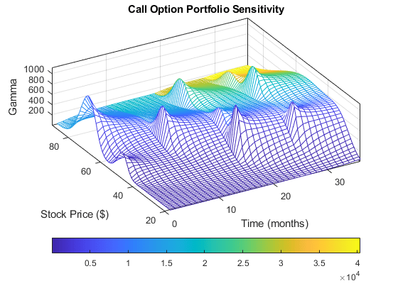
This example plotsgammaas a function of price and time for a portfolio of ten Black-Scholes options.

The plot in this example shows a three-dimensional surface. For each point on the surface, the height (z-value) represents the sum of the gammas for each option in the portfolio weighted by the amount of each option. Thex-axis represents changing price, and they-axis represents time. The plot adds a fourth dimension by showing delta as surface color. This example has applications in hedging. First set up the portfolio with arbitrary data. Current prices range from $20 to $90 for each option. Then, set the corresponding exercise prices for each option.

Range = 20:90; PLen = length(Range); ExPrice = [75 70 50 55 75 50 40 75 60 35];

设置所有无风险利率至10%,times to maturity in days. Set all volatilities to 0.35. Set the number of options of each instrument, and allocate space for matrices.

Rate = 0.1*ones(10,1); Time = [36 36 36 27 18 18 18 9 9 9]; Sigma = 0.35*ones(10,1); NumOpt = 1000*[4 8 3 5 5.5 2 4.8 3 4.8 2.5]; ZVal = zeros(36, PLen); Color = zeros(36, PLen);

For each instrument, create a matrix (of sizeTimebyPLen) of prices for each period.

fori = 1:10 Pad = ones(Time(i),PLen); NewR = Range(ones(Time(i),1),:);

Create a vector of time periods1toTimeand a matrix of times, one column for each price.

T = (1:Time(i))'; NewT = T(:,ones(PLen,1));

Use the Black-Scholes gamma and delta sensitivity functionsblsgammaandblsdeltato computegammaanddelta.

ZVal(36-Time(i)+1:36,:) = ZVal(36-Time(i)+1:36,:)...+ NumOpt(i) * blsgamma(NewR, ExPrice(i)*Pad,...Rate(i)*Pad, NewT/36, Sigma(i)*Pad); Color(36-Time(i)+1:36,:) = Color(36-Time(i)+1:36,:)...+ NumOpt(i) * blsdelta(NewR, ExPrice(i)*Pad,...Rate(i)*Pad, NewT/36, Sigma(i)*Pad);end

Draw the surface as a mesh, set the viewpoint, and reverse thex-axis because of the viewpoint. The axes range from20to90,0to36, and -∞ to ∞.

mesh(Range, 1:36, ZVal, Color); view(60,60); set(gca,'xdir',“反向”,'tag','mesh_axes_3'); axis([20 90 0 36 -inf inf]);

Add a title and axis labels and draw a box around the plot. Annotate the colors with a bar and label the color bar.

title('Call Option Portfolio Sensitivity'); xlabel('Stock Price ($)'); ylabel('Time (months)'); zlabel('Gamma'); set(gca,'box','on'); colorbar('horiz');

See Also

bnddury|bndconvy|bndprice|bndkrdur|blsprice|blsdelta|blsgamma|blsvega|zbtprice|zero2fwd|zero2disc|corr2cov|portopt

Related Topics

• Plotting Sensitivities of an Option
• Pricing and Analyzing Equity Derivatives
• Greek-Neutral Portfolios of European Stock Options
• Sensitivity of Bond Prices to Interest Rates
• Bond Portfolio for Hedging Duration and Convexity
• Bond Prices and Yield Curve Parallel Shifts
• Bond Prices and Yield Curve Nonparallel Shifts
• Term Structure Analysis and Interest-Rate Swaps